Following on from the previous post looking at methods for identifying overhang regions for use in support structures, the ray projection method approached felt unsatisfactory, especially from a performance perspective. This is used as part of the support generation module when determining self-intersecting support structures with the part and for generating the initial 3D conformal volumetric block supports alongside the boolean operations.
The depth projection map is used to firstly identify the unsupported regions, using the selecting overhang angle. These regions are then intersected with the existing part to detect self-intersection and those regions that are only attached to the build-plate. This is later determined by seperate support volumes by identifying large differences between the region. This will be later explained in greater detail in a following post.
The in-built ray projection method used by Trimesh used the RTree library internally. Alternatively, PyEmbree, based on Intel’s Embree library can be used, although extremely efficient for purposes of RayTracing application, it unfortunatly cannot provide an accurate ray intersection for the purposes of generating support structures. The Rtree method unfortunately is not particularly high performance, even using a spatial tree-index structure for the acceleration structure and is also not multi-threaded. Increasing the resolution spatially has a performance cost O(\Delta x^2) and this is ultimately linear based on the number of ray search. Increasing the complexity of the mesh and throwing more triangles into the mix, further compounds the computational effort. Anecdotally, this mirrors the same issue with some voxelisation methods based on ray-tracing methods such as the one proposed by A. Aitkenhead .
The previous solution worked, especially on relatively simple geometries, but was unsatisfactory even with a boolean intersection with the a mesh created projecting the support surface downwards.
Following a foray into learning about GPU computing using GLSL shaders and also OpenCL and two years ago, there seemed a practical approach to solving this. This similar approach has also been recently used for generating signed-distance fields for meshes for use in Deep Learning geometries in PyTorch3D, shared on their Github repo. Their approach projects points close to the mesh and then using the surface normals and native depth occlusion tests available in OpenGL can project an approximate signed distance field – this has now become abbreviated (SDF) in literature.
Methodology
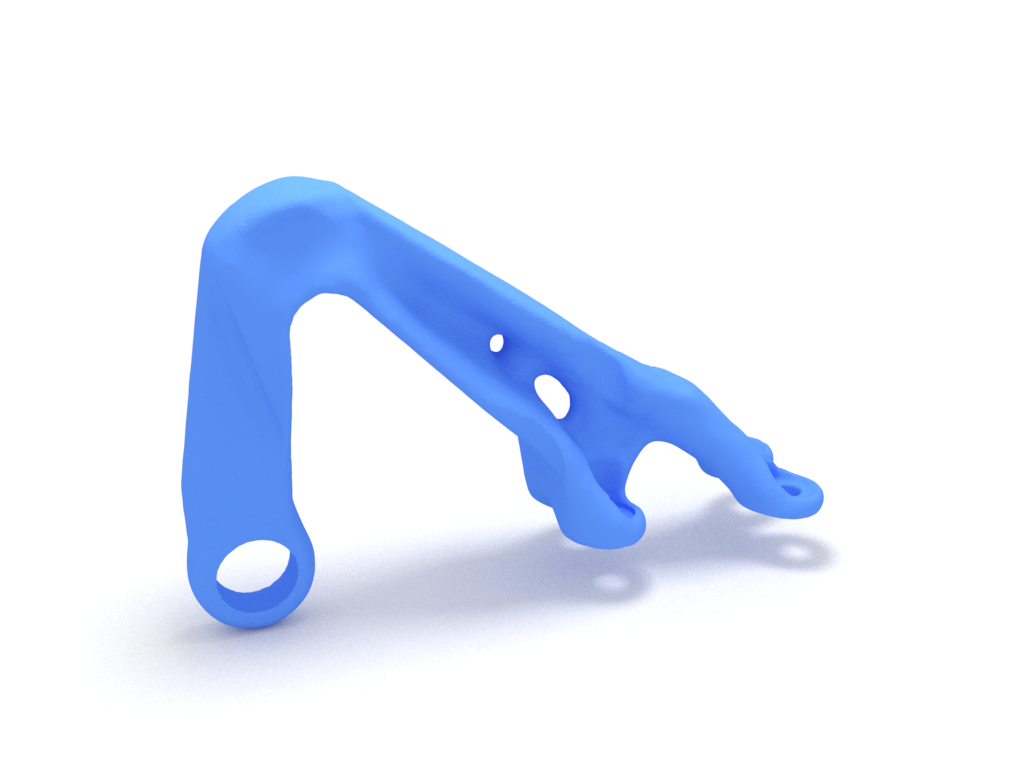
For illustrating the method, the existing geometry of a topology optimised bracket to demonstrate a relatively dense triangular mesh, the part is orientated in the following fashion.
Like the previous method, we do not necessarily have to work with the overhang region mesh.
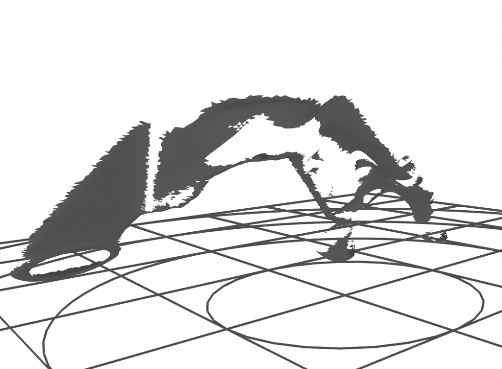
In the method, one simply needs to rasterise the Z-position of the surface of the mesh and discard hidden surfaces in order to emulate a single-hit ray projection approach. Using OpenGL GLSL fragment shaders this can be done by taking the orthographic projection of the model and then rasterising the Z position of each fragment (pixel) across each triangle.
The occlusion test is natively built into the standard 3D Graphics pipeline, which essentially emulates the ray-tracing approach. As trivial as it may sound, programming this in Python didn’t come easy. It required changing the framebuffer object (images that the triangles are rendered). Another subtle trick required is defining the the vertex colour Vertex Buffer Object (VBO) with the z-coordinates for its corresponding triangle vertex. The Z ‘colour’ value is then natively interpolated across each triangle during rasterisation and based on the depth-test performed automatically by OpenGL, only the most closest value remains, with other fragments in discarded. The GLSL fragment shader is shared below:
# Vertex shader

/ Uniforms
// ------------------------------------
uniform   mat4 u_model;
uniform   mat4 u_view;
uniform   mat4 u_projection;
uniform   vec4 u_color;

// Attributes
// ------------------------------------
attribute vec3 a_position;
attribute vec4 a_color;
attribute vec3 a_normal;

varying vec4 v_color;

void main()
{
    v_color = a_color;// * u_color;
    gl_Position = u_projection * u_view * u_model * vec4(a_position,1.0);
}

# Fragment shader
varying vec4 v_color;
out vec4 fragColor;

void main()
{
    fragColor = vec4(v_color.z,v_color.z,v_color.z,1.0);
}
The desired resolution of the ray-projection map is simply changed by setting the Window size or the underlying framebuffer size. The implementation is based on Vispy library, which provides access to many low-level building-blocks for creating OpenGL applications via its supporting library Glumpy. In this implementation, the vispy.app.Canvas is redefined , including the GLSL Shader Programs, OpenGL transformation matrices (Model-View-Projection MVP matrices) and also the framebuffer properties and OpenGL states required for rendering the mesh.
class Canvas(app.Canvas):

    def __enter__(self):
        self._backend._vispy_warmup()
        return self

    def __init__(self, rasterResolution  = 0.02):

        self.vertices, self.filled, self.verticesColor, part = meshPart()

        vertex_data = np.zeros(self.vertices.shape[0], dtype=[('a_position', np.float32, 3),
                                                              ('a_color', np.float32, 3)])

        vertex_data['a_position'] = self.vertices.astype(np.float32)
        vertex_data['a_color'] = self.vertices.astype(np.float32)

        meshbbox = part.geometry.bounds
        self.box = meshbbox
        meshExtents = np.diff(meshbbox, axis=0)

        resolution = 0.05
        visSize = (meshExtents / resolution).flatten()
        self.visSize = visSize

        app.Canvas.__init__(self, 'interactive',  show=False, autoswap=False, size=(visSize[0], visSize[1]))

        self.filled = self.filled.astype(np.uint32).flatten()
        self.filled_buf = gloo.IndexBuffer(self.filled)

        self.program = gloo.Program(vert, frag)
        self.program.bind(gloo.VertexBuffer(vertex_data))

        avg = np.mean(self.box, axis=0)

        self.view = rotate(0, [1,0,0]) #translate([0,0,0])
        self.model = np.eye(4, dtype=np.float32)

        print('Physical size:', self.physical_size)

        shape = self.physical_size[1], self.physical_size[0]

        self._rendertex = gloo.Texture2D((shape + (4,)), format='rgba', internalformat='rgba32f')
        self._depthRenderBuffer = gloo.RenderBuffer(shape, format='depth')
        self._depthRenderBuffer.resize(shape, format=gloo.gl.GL_DEPTH_COMPONENT16)

        # Create FBO, attach the color buffer and depth buffer
        self._fbo = gloo.FrameBuffer(self._rendertex, self._depthRenderBuffer)

        gloo.set_viewport(0, 0, self.physical_size[0], self.physical_size[1])
        self.projection = perspective(45.0, self.size[0] /
                                      float(self.size[1]), 2.0, 10.0)

        self.projection = ortho(self.box[1, 0], self.box[0, 0], self.box[1, 1], self.box[0, 1], 2, 40)

        self.program['u_projection'] = self.projection

        self.program['u_model'] = self.model
        self.program['u_view'] = self.view

        self.theta = 0
        self.phi = 0

        gloo.set_clear_color('white')
        gloo.set_state('opaque')
        gloo.set_polygon_offset(1, 1)

        self.update()

    def on_timer(self, event):
        self.theta += .5
        self.phi += .5
        self.model = np.dot(rotate(self.theta, (0, 1, 0)),
                            rotate(self.phi, (0, 0, 1)))
        self.program['u_model'] = self.model

        self.update()

    def setModelMatrix(self, model):
        self.model = np.dot(rotate(self.theta, (0, 1, 0)),
                            rotate(self.phi, (0, 0, 1)))
        self.program['u_model'] = self.model
        self.update()

    def on_resize(self, event):
        from vispy.util.transforms import perspective, translate, rotate, ortho

        gloo.set_viewport(0, 0, event.physical_size[0], event.physical_size[1])
        # Create the orthographic projection
        self.projection = ortho(self.box[1, 0], self.box[0, 0],
                                self.box[1,1], self.box[0, 1],
                                -self.box[1, 2], self.box[0, 2])
        self.program['u_projection'] = self.projection

    def on_draw(self, event):

        from vispy.util.transforms import perspective, translate, rotate, ortho
        from vispy.gloo.util import _screenshot

        with self._fbo:
            gloo.clear()
            gloo.set_clear_color((0.0, 0.0, 0.0, 0.0))
            gloo.set_viewport(0, 0, *self.physical_size)
            gloo.set_state(blend=False, depth_test=True, polygon_offset_fill=False)
            self.program['u_color'] = 1, 1, 1, 1
            self.program.draw('triangles', self.filled_buf)
            #self.rgb = np.copy(self._fbo.read('color')) #_screenshot((0, 0, self.size[0], self.size[1]))  #self._fbo.read('color')
            #self.rgb =     gloo.read_pixels((0, 0, *self.physical_size), True)
            self.rgb  = _screenshot((0, 0, *self.physical_size))

c = Canvas()
c.show(visible=True)
Once complete, the output from the framebuffer can then be transferred to a numpy array for further processing. Very large resolutions may be achieved with little performance impact using GPU computation. These high resolution ray-projection maps are extremely important for accurately capturing the overhang regions and ensuring that each support structure is correctly attached and conforming to the part’s geometry.
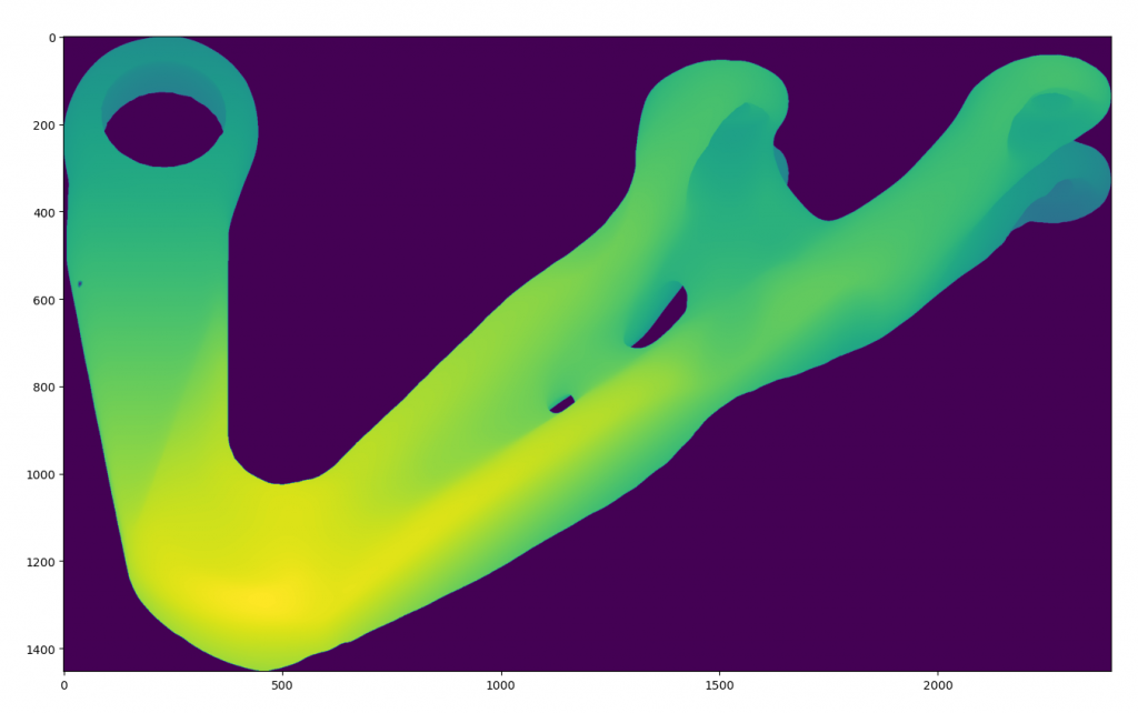
Another advantage of capturing the effective ray projection using this means, is the background is clearly identified easing segmentation. Upon obtainingt the ray-projection method, the overhang regions can be identified as using the gradient of the ray project map, as discussed in the previous post. Gaussian convolution kernel may be applied on the thresholded image, so that the boundaries can be smoothed before extracting boundaries.
The boundaries may then be obtained using by extracting the isolevel from the thresholded image accordingly using
import skimage.measure
import skimage.filters
import pyslm.visualise
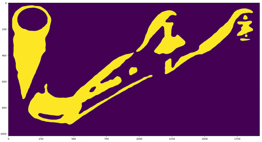
# The background is masked using the alpha channel from the framebuffer. A gaussian blur is applied onto the overhang image to smoothen boundaries
ov = overhang * c.rgb[:,:,3]
ov = skimage.filters.gaussian(ov, sigma=8)
plt.imshow(ov > 0.5)
# Locate the boundaries using marching-squares algorithm
contours = skimage.measure.find_contours(ov.T, 0.5)
# Create the paths for manipulation later
fig = plt.figure()
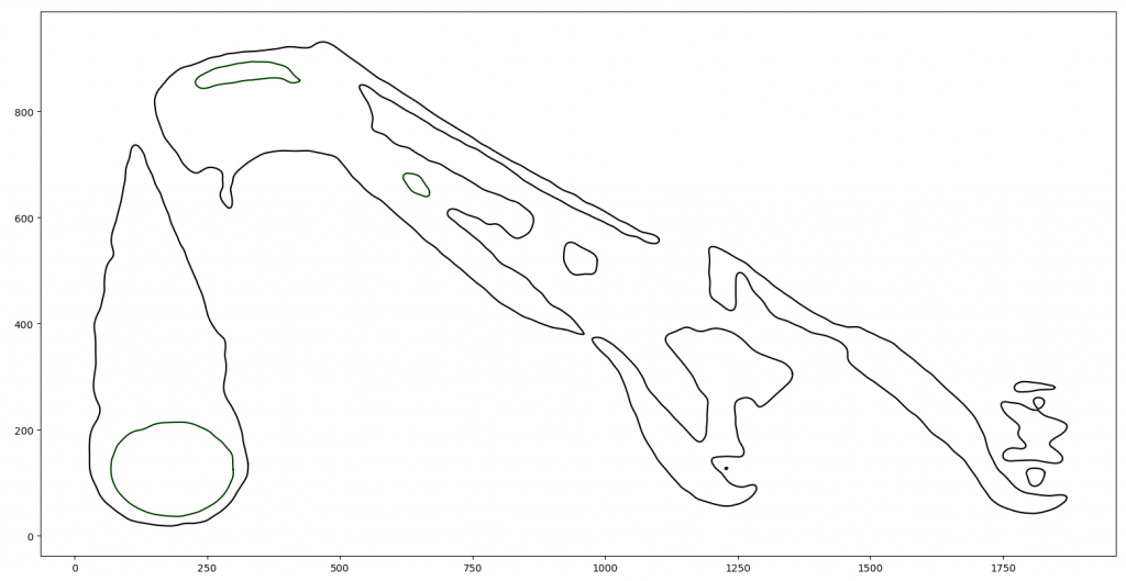
triPath = pyslm.support.createPath2DfromPaths(contours)The resultant boundaries are shown below.
Conclusions
Despite the simplicity of this method, it is not readily used in many areas despite its advantages. The problem with the method is often setting up a suitable OpenGL environment and back-end in Windows and Linux environments, especially in conjunction with using Python. This resulted in many delays in the release of PySLM v0.5, but these have been resolved across all platforms.
This approach provides a very fast and efficient method for performing ray-projection tests especially resolving this at high resolutions for complex meshes harnessing the power of GPUs. Having a complete rasterised image with polygon boundaries provides the ability to offset and generate smoother support regions later.
See the Next Post in the Series