The in-built visualisation for scan paths in PySLM leverages matplotlib – refer to a previous post. This is sufficient for most user’s needs when attempting to interpret and visualise the scan paths generated in PySLM, or those imported from a slice taken from an existing machine build files. Extending this beyond multiple layers or large parts becomes more tricky when factoring in visualisation of some parameters (e.g. Laser Power, effective scan speed). Admittedly, the performance of Matplotlib becomes limited to explore the intricacies and complexities embedded within the scan vectors.
For scientific research, the fusion of scan vector geometry with volumetric datasets such as X-Ray CT during post-inspection of parts/samples, or those generated within the build process including pyrometry data, thermal-imaging offer the ability to increase our understanding and insight to observations of the effect of process on the material produced using L-PBF. GPU based visualisation libraries such (vispy) would offer the possibility to accelerate the performance, but are not user-friendly nor offer interactivity when manipulating views and the data and are often cumbersome when processing volumetric datasets often encountered in Additive Manufacturing. Paraview is a cross-platform open-source scientific visualisation tool that is especially powerful for processing, interaction and visualisation of large-scale scientific datasets.
Paraview and the underlying VTK library offers an alternative ready-made solution to visualise this information, and are most importantly hardware accelerated with the option for raytracing provided by OSPRay and OptiX for latest RTX NVIDIA cards that include Raytracing (RT) cores. Additionally, the data can be augmented and processed using parallelised filters and tools in Paraview.
VTK File Format
Ignoring the HDF5 variations that are most useful for structured data, the underlying format within vtk that used for storing vector based data and point cloud data is the .vtp file format. The modern VTK file formats use an XML schema – unlike the legacy format, to store a structured series of geometry (volumetric data, lines, polygons, 3D elements and point clouds). The internal data format can be stored using ascii encoding or binary. Binary data can be incorporated directly within a parsable .xml format using a Base64 encoding and may additional incorporate internal compression. Alternatively data can be stored in an appended data section located at the footer of the file, which treats data section as a contiguous block of raw data. Different sub-formats exist, that are appropriate for different types of data e.g. volumetric, element based (Finite Volume / Finite Element derived) or polygon based. An approach relevant to export scan vector geometry the .vtp – format is most suitable.
The data stored in the VTK Point file consists of:
3D points coordinates
Data attributes stored at each point location
Geometric elements (lines, polygons) defining connectivity with reference to the list of point coordinates
Paraview exporter implementation:
The Paraview exporter is simplistic, because the data compression is currently ignored. The process is similar to the technique used in the function pyslm.visualise.plotSequential, whereby hatch and contour vectors are merged and reprocessed in order that they represent always a series of lines (an n x 2 x 2 array). This is not the most efficient option for ContourGeometry (border scans) where scan vectors are continuously joined up, but simplifies the processing working with the data.
Once the scan vector coordinates and the relevant data are packaged up into a single array, the data is wrote within the sub-sections of the XML file. Data is stored using floating points or integers accordingly in a binary representation. The data used to represent coordinates and indices for each vector, are stored with the ‘appended’ option within the <DataArray> element of each section. The raw data is stored and collected that are then written in the <AppendedData> element at the end of file with raw encoding option chosen. The byte offsets for the position of each ‘chunk’ of data that are referenced by the <DataArray> element are collected and stored incrementally.
For reference, the following information is provided for writing raw data, because this was difficult to obtain from the VTK documentation directly.
<AppendedData encoding=”raw”>
Start of Raw Data Section
_
Underscore character is starting location for reading raw data
Section Size (Int32/Int64)
Integer representing size of following section (include the size in bytes with the offsets provided). The integer type should match the size used in the header.
Raw data (e.g Int32, float32, float64)
….
Repeated the above (two rows) for each referenced data section
</AppendedData>
Example Scan Vector Data exported to VTK
An example Aconity .ILT file was imported into PySLM and then exported to a .vtp VTK file that was processed in Paraview. The scan order is visualised by the colour map with each vertex assigned a global-id. The ‘Tube‘ filter was applied to each scan vector in order to improve their visibility.
The script excerpt can currently be found on a Gist. This will be later included in future versions of PySLM along with other import/exporters.
Following on from the previous post in Part II, this post will detail the methodology for ‘Grid Block’ support generation, which is one of the most commonly utilised support structure used especially in the selective laser melting process.
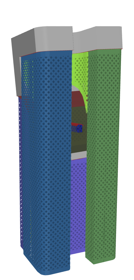
The definition of a volumetric block support region is illustrated shown below for an example topology optimised bracket. These are projected volume regions that extend vertically dowwards from the original overhang surface, that conforms exactly with the input mesh.
Volume Block Support Structures extruded from overhang un-supported regions for a topology optimised bracket
Prior to starting this work, two approaches for generating ‘block‘ based support structures seem to exist. However, these approaches did not seem satisfactory especially when it came to their use using cost models.
The first approach identified, typically employed in FDM based processes, obtains the support or overhang regions and then generated a 2D polygon region that is the flattened or projection of this surface. The polygon is incrementally generated for each slice layer and a combination of boolean operations and offsetting operations are used to detect self intersections with existing geometry to modify its shape. It’s a robust method and can generate support features to aid manufacturing. The limitation of this approach is it cannot generate a volume, or an explicit mesh geometry. Rather a discretionary of the geometry containing slices representing the region with a sparse infill.
The second approach would appear to voxelise or generates a levelset of the geometry. Under support regions, the voxel grid is filled to create the in-fill support regions. The volume region can be re-constructed into a support structure and a truss structure can be generated inside. This method is not able to generate clean meshes of the support volume and requires a discretisation of the original geometry.
The following method proposed uses a hybrid mesh approach in order to generate clean meshes using fairly conventional boolean CSG library. The actual support structure generated uses relies on using 2D polygons to generate complex features such as perforation holes or structures.
Overall Support Module Structure Summary
The overall support module, in its current state for version 0.5, is split into the following structure. The generation of supports is performed by a utility ‘generator‘ class BaseSupportGenerator and incidentally their derived classes:
These classes perform the overhang and support analysis to extract the overhang surfaces. From the overhang surface, the support volumes are then generated using these to provide the inputs used to generate specific support objects that may have a specific style. For the objects representing the actual support structures, and regions, these are split into the following classes:
SupportStructure – Base class defining a part’s surface requiring support
BlockSupportBase – Generates support block volumes for providing a region to support
GridBlockSupport– Generates a support with a grid trust suitable for SLM
Overhang and Support Area Identification
The first step, widely available amongst all CAD and pre-processing software is overhang identification. Determining the face angles is a trivial process and in PySLM may be obtained using the following function pyslm.support.getSupportAngles. The function takes the trimesh object and calculates the dot product of the surface normal across the mesh. Upon obtaining the dot product, the angle between the vectors is calculated and for convenience is converted from rads to degrees. Further explanation is provided in a previous post.
# Normal to the Z Plane
v0 = np.array([[0., 0., -1.0]])

#Identify Support Angles
v1 = part.geometry.face_normals

# Calculate the angle (degrees) between the face normals and the Z-plane
theta = np.arccos(np.clip(np.dot(v0, v1.T), -1.0, 1.0))
theta = np.degrees(theta).flatten()
Upon obtaining the surface angles, the overhang mesh regions can be extracting from the originating mesh, similar to that used in pyslm.support.getOverhangMesh. A comparison to a threshold overhang or support angle is made and used as a mask to extract the face indices from the mesh in order to obtain a new mesh. It is common that the overhang regions are disconnected. These can optionally be split using trimesh.split , which uses the internal connectivity of vertices in the mesh in a connected-component algorithm to isolate separate regions.
# Extract a list of faces that are below the critical overhangeAngle specified
supportFaceIds = np.argwhere(theta > 180 - overhangAngle).flatten()

# Create the overhang mesh by splitting the meshing when needed.
overhangMesh = trimesh.Trimesh(vertices=part.geometry.vertices,
                               faces=part.geometry.faces[supportFaceIds])
if splitMesh:
    return overhangMesh.split(only_watertight=False)
Splitting the mesh is far more convenient in terms of processing the support structures. It also improves the performance by reducing the projected area when performing ray intersections to identify an approximate volume.
Providing a robust method for obtaining the projected support volume is not a straightforward task, especially without sophisticated boolean operation tools. Through some experimentation with the given software libraries available, the following process offered a satisfactory result without a reasonably long computational cost.
Summary of method
The following operations are performed to generate block supports:
Support regions (3D mesh surface) are separated into meshes
Each support region mesh is flattened into a polygon and the contour is offset
Surface region is extruded to z=0
Intersection test using a Boolean Mesh Intersection operation is performed to check if self-intersection with part
If self-intersection exist a ray-projection height map is created
Side surfaces are removed from the intersection
Ray projections are made separately on upward facing and downward facing faces and the height map is built up
The gradient of the height-map is used to separate regions are extracted outlines of separate support regions
For each support region:
Triangulate the polygon regions into a mesh
Rays are projected along Z in both directions from the mesh vertices to obtain the required extrusion height
The triangulated polygon is extruded in both directions using the extrusions heights with an offset
The extruded prisms are intersected with the original part mesh to obtain the final support volumes.
Inside the function, the support regions are flattened into a polygon BaseSupportGenerator.flattenSupportRegion. This method extracts the outline or the boundary of the support region and flattens via projection by setting z=0along the coordinates. The paths are then translated into Shapely.Polygon objects.
""" Extract the outline of the overhang mesh region"""
poly = supportRegion.outline()

""" Convert the line to a 2D polygon"""
poly.vertices[:, 2] = 0.0

flattenPath, polygonTransform = poly.to_planar()
flattenPath.process()

flattenPath.apply_translation(polygonTransform[:2, 3])
polygon = flattenPath.polygons_full[0]
The polygon region is generated it provides the elementary building block for generating a support structure. This can be used to offset to prevent collision with self intersecting features. Internally, offsetting is useful to perform to regions so that any self-intersections with the geometry are clean.
Region Extrusion and Self-Intersection Check
The first pass of the proposed algorithm requires performing a boolean intersection to identify if there are any self-intersections. The polygon regions require extrusion. Near-net shape extrusion is accomplished using a custom function pyslm.support.extrudeFace. Unfortunately, this is not available within Trimesh, so instead it had to be implemented manually. This function extrudes a region of connected faces within a polygon, to set position or each individual face offset by an extruded distance.
# Extrude the surface to Z = 0
extrudedBlock = extrudeFace(supportSurface, None, 0)

# Extrude a triangle surface (Trimesh) based on the heights corresponding to each surface triangle
extrudedBlock = extrudeFace(surface, None, heightArray)
Having obtained an extruded prism from the support surface, a self-intersection test is performed with the original part. If no self-intersection takes place, this means the support structure has connectivity with the build platform. Under this situation, this drastically simplifies the number of steps required.
Example of an extruded mesh used for self-intersection tests
The intersection test requires a Boolean CSG operation. Quickly profiling a couple of tools available, from experience trying available solutions, the Cork Library was found to be both a reasonably accurate and high performance tool for manifold 3D geometries (i.e. those already required for 3D printing). The Nef Polyhedra implementation in the CGal library is renowned to be an accurate and robust implementation but slow. Due to these reasons, the PyCork library was created to provide a convenient wrapper across all platforms to perform this.
# Below is the expanded intersection operation used for intersecting a mesh
# cutMesh = pyslm.support.geometry.boolIntersect(part.geometry, extrudedMesh)

meshA = part.geometry
meshB = extrudedMesh

vertsOut, facesOut = pycork.intersection(meshA.vertices, meshA.faces, meshB.vertices, meshB.faces)

# Re-construct the Trimesh
cutMesh = trimesh.Trimesh(vertices=vertsOut, faces=facesOut, process=True)

# Identify if there is a self-intersection
if cutMesh.volume < BlockSupportGenerator._intersectionVolumeTolerance: # 50
    # The support does not self intersect
else:
    # The support intersects with the original part
In the situation that there is no intersection (or the volume is approximately zero), the support volume simply extrudes towards the build-plate. If a self-intersection occurs with the part, further calculations are required to process the block support.
Self-Intersecting Support Structures
If the support-self intersects this is far more challenging problem to deal with. Through a lot of experimentation, the most reliable method determined involved using a form of ray-tracing to project the surfaces down. This has two benefits:
Separating support regions across different heights
Providing a robust method for generating cleaner support volumes with greater options to customise their behaviour
The ray projection test is useful generally, as it can also be used to provide a support generation map for the region, as shown in the previous post.
Originally the ray projection method was done using Trimesh.Ray, where rays are projected from each support face at a chosen ray projection resolution BlockSupportGenerator.rayProjectionResolution. A grid is formed with seed points for the rays and these are projected upwards and downwards onto the previous self intersected support mesh. The ray intersection test is performed on upward facing surfaces extracted from the existing intersected mesh, in the previous region.
Later this was updated to use a GLSL GPU process for identifying this at a much higher resolution at significant reduction in computational cost as discussed in a previous post.
From the ray projection map, individual support block regions can be separated based on taking a threshold of the image gradient, using the gradThreshold function. Using simple trigonometry, the threshold to determine disconnected regions in the intersecting support are determined by the resolution of the ray projected image and the overhang angle, with an added ‘fudge-factor‘ thrown in.
Regions are separated based on this threshold using the isocontour method offered in Skimage’sfind_contours function. This is useful because it can identify supports regions connected only to the build-platform (desirable) and self-intersecting regions with the original part. Additionally, self-intersecting support regions with difference heights can also be isolated. These are useful in some marginal scenarios, but were more simpler methods breakdown.
Ray Projection Map of support region used for identifying and separating support regions. Note the relatively high resolution used by using the GPU Projection Map Technique
A projected region extracted by extracting the contour isolevel from the projection map (left). The outline is transformed into absolute coordinate system for the part.
The regions are identified by taking a threshold based on the choice of overhang angle using the BlockSupportGenerator.gradThreshold.
def gradThreshold()
    return 5.0 * np.tan(np.deg2rad(overhangAngle)) * rayProjectionDistance

# Calculate the gradient of the ray-projected height map for the support region
vx, vy = np.gradient(heightMap)
grads = np.sqrt(vx ** 2 + vy ** 2)

# A blur is used to smooth the boundaries
grads = scipy.ndimage.filters.gaussian_filter(grads, sigma=BlockSupportGenerator._gausian_blur_sigma)

"""
Find the outlines of any regions of the height map which deviate significantly
"""
outlines = find_contours(grads, self.gradThreshold(self.rayProjectionResolution, self.overhangAngle),
                            mask=heightMap > 2)

# Transform the outlines from image to global coordinates system
outlinesTrans = []
for outline in outlines:
    outlinesTrans.append(outline * self.rayProjectionResolution + bbox[0, :2])
Once the outlines are obtained. The boundaries are created into polygons, offset, optionally smoothed and then translated into triangular meshes using triangulate_polygon. Care must be taken when using spline-fitting to smooth the boundary as this can result in profiles not conforming to the original overhang region. The triangulation procedure internally can use either the earbox-cut algorithm or constrained Delaunay via the Triangle Library. The points of the polygon mesh are projected upwards and downwards on a subset of the previous intersected mesh to located the approximate volume before performing the final boolean operation.
# Create the outline and simplify the polygon using spline fitting (via Scipy)
mergedPoly = trimesh.load_path(outline)
mergedPoly.merge_vertices(1)

# Simplification and smoothing of the boundary is perform to provide smoother boundaries for generating a truss structure later.
mergedPoly = mergedPoly.simplify_spline(self._splineSimplificationFactor)

outPolygons = mergedPoly.polygons_full

"""
Triangulate the polygon into a planar mesh
"""
poly_tri = trimesh.creation.triangulate_polygon(bufferPoly, triangle_args='pa{:.3f}'.format(self.triangulationSpacing))

# Use a ray projection method onto the original geometry to identify upper and lower boundaries

coords = np.insert(poly_tri[0], 2, values=-1e-7, axis=1)
ray_dir = np.repeat([[0., 0., 1.]], coords.shape[0], axis=0)

# Find the first location of any triangles which intersect with the part
hitLoc, index_ray, index_tri = subregion.ray.intersects_location(ray_origins=coords,
                                                                    ray_directions=ray_dir,
                                                                    multiple_hits=False)
The same process is repeated, and an extruded prism is generated based on the ray-projection regions. Simplification of the interior triangulation is done in order to minimise the time to perform the intersection.
The prismatic mesh extruded based on the ray-projection distances obtained.
The prismatic mesh extruded based on the ray-projection distances obtained.
Finally, to obtain the ‘exact’ conforming intersected mesh, once again this is intersected with the previous mesh to obtain the final support volume region conforming to the original geometry.
As it can be observed, there are many steps to obtain the exactly conforming support volume with the original mesh. For the majority of most geometries that would be printed, this method is adequate, although not full-proof. There are a few cases where this algorithm will fail due to the use of a ray projection algorithm and relying on line-of-sight. For example, a continuous spiral or 3D helix structure with large connected surfaces will not be identifiable from the support generation algorithm. Without developing a specific mesh intersection library, it is difficult to identify alternative ways around this. Admittedly this is beyond my ability.
Following on from the previous post looking at methods for identifying overhang regions for use in support structures, the ray projection method approached felt unsatisfactory, especially from a performance perspective. This is used as part of the support generation module when determining self-intersecting support structures with the part and for generating the initial 3D conformal volumetric block supports alongside the boolean operations.
The depth projection map is used to firstly identify the unsupported regions, using the selecting overhang angle. These regions are then intersected with the existing part to detect self-intersection and those regions that are only attached to the build-plate. This is later determined by seperate support volumes by identifying large differences between the region. This will be later explained in greater detail in a following post.
The in-built ray projection method used by Trimesh used the RTree library internally. Alternatively, PyEmbree, based on Intel’s Embree library can be used, although extremely efficient for purposes of RayTracing application, it unfortunatly cannot provide an accurate ray intersection for the purposes of generating support structures. The Rtree method unfortunately is not particularly high performance, even using a spatial tree-index structure for the acceleration structure and is also not multi-threaded. Increasing the resolution spatially has a performance cost O(\Delta x^2) and this is ultimately linear based on the number of ray search. Increasing the complexity of the mesh and throwing more triangles into the mix, further compounds the computational effort. Anecdotally, this mirrors the same issue with some voxelisation methods based on ray-tracing methods such as the one proposed by A. Aitkenhead .
The previous solution worked, especially on relatively simple geometries, but was unsatisfactory even with a boolean intersection with the a mesh created projecting the support surface downwards.
Following a foray into learning about GPU computing using GLSL shaders and also OpenCL and two years ago, there seemed a practical approach to solving this. This similar approach has also been recently used for generating signed-distance fields for meshes for use in Deep Learning geometries in PyTorch3D, shared on their Github repo. Their approach projects points close to the mesh and then using the surface normals and native depth occlusion tests available in OpenGL can project an approximate signed distance field – this has now become abbreviated (SDF) in literature.
Methodology
For illustrating the method, the existing geometry of a topology optimised bracket to demonstrate a relatively dense triangular mesh, the part is orientated in the following fashion.
Topology optimised bracket used as an example for identifying support regions using a ray projection method.
Like the previous method, we do not necessarily have to work with the overhang region mesh.
The extracted overhang mesh obtained from a Topology Optimised Bracket
In the method, one simply needs to rasterise the Z-position of the surface of the mesh and discard hidden surfaces in order to emulate a single-hit ray projection approach. Using OpenGL GLSL fragment shaders this can be done by taking the orthographic projection of the model and then rasterising the Z position of each fragment (pixel) across each triangle.
The occlusion test is natively built into the standard 3D Graphics pipeline, which essentially emulates the ray-tracing approach. As trivial as it may sound, programming this in Python didn’t come easy. It required changing the framebuffer object (images that the triangles are rendered). Another subtle trick required is defining the the vertex colour Vertex Buffer Object (VBO) with the z-coordinates for its corresponding triangle vertex. The Z ‘colour’ value is then natively interpolated across each triangle during rasterisation and based on the depth-test performed automatically by OpenGL, only the most closest value remains, with other fragments in discarded. The GLSL fragment shader is shared below:
The desired resolution of the ray-projection map is simply changed by setting the Window size or the underlying framebuffer size. The implementation is based on Vispy library, which provides access to many low-level building-blocks for creating OpenGL applications via its supporting library Glumpy. In this implementation, the vispy.app.Canvas is redefined , including the GLSL Shader Programs, OpenGL transformation matrices (Model-View-Projection MVP matrices) and also the framebuffer properties and OpenGL states required for rendering the mesh.
Once complete, the output from the framebuffer can then be transferred to a numpy array for further processing. Very large resolutions may be achieved with little performance impact using GPU computation. These high resolution ray-projection maps are extremely important for accurately capturing the overhang regions and ensuring that each support structure is correctly attached and conforming to the part’s geometry.
Output generated from Vispy to rasterise the Z-position to emulate the ray-projection method. Note the high resolution attainable using this approach. The only limitation is the size of the GPU framebuffer.
Another advantage of capturing the effective ray projection using this means, is the background is clearly identified easing segmentation. Upon obtainingt the ray-projection method, the overhang regions can be identified as using the gradient of the ray project map, as discussed in the previous post. Gaussian convolution kernel may be applied on the thresholded image, so that the boundaries can be smoothed before extracting boundaries.
Overhang angles obtained based on the gradient across the depth image and a threshold.
The boundaries may then be obtained using by extracting the isolevel from the thresholded image accordingly using
import skimage.measure
import skimage.filters
import pyslm.visualise

# The background is masked using the alpha channel from the framebuffer. A gaussian blur is applied onto the overhang image to smoothen boundaries
ov = overhang * c.rgb[:,:,3]
ov = skimage.filters.gaussian(ov, sigma=8)

plt.imshow(ov > 0.5)

# Locate the boundaries using marching-squares algorithm
contours = skimage.measure.find_contours(ov.T, 0.5)

# Create the paths for manipulation later
fig = plt.figure()
triPath = pyslm.support.createPath2DfromPaths(contours)
The resultant boundaries are shown below.
Boundaries extracted from the overhang regions. The boundaries may be simplified later.
Conclusions
Despite the simplicity of this method, it is not readily used in many areas despite its advantages. The problem with the method is often setting up a suitable OpenGL environment and back-end in Windows and Linux environments, especially in conjunction with using Python. This resulted in many delays in the release of PySLM v0.5, but these have been resolved across all platforms.
This approach provides a very fast and efficient method for performing ray-projection tests especially resolving this at high resolutions for complex meshes harnessing the power of GPUs. Having a complete rasterised image with polygon boundaries provides the ability to offset and generate smoother support regions later.
A key focus of the release of PySLM 0.5 was the introduction of support structure generation targeted for powder-bed fusion (PBF) processes such as Selective Laser Melting (SLM) and also Electron Beam Melting (EBM). The basic infrastructure for generating support structures was developed including overhang analysis, support projection maps and the calculating precise conforming volumes, that leads to demonstration of block ‘truss’ based supports.
It is a particularly exciting release, because it is the first implementation both open source but also explicitly documents in practice a potential method for generating support structures for these specific PBF processes that have commercially (albeit few choices) been available for over a decade.
The challenge of this specific problem was to provide a robust solution covering the majority of engineering cases – which led to the length of time taken to develop this feature. This included having to develop many additional functions, support routines and workarounds for the limited availability of a boolean CSG library for triangular meshes in Python whilst providing reasonable performance.
In the Support Structure, the geometry constructed consists of a grid and a boundary which features a polygon derived truss structure in order to support powder removal and control the stiffness of the structure. Below highlights the capability for generated truss-based support structure suitable for PBF process. Carefully observe that individual support blocks are separated when self-intersecting and precisely conform to the original geometry. The support volumes themselves interface with the original part, by performing an exact boolean intersection.
Support Structure Generation in PySLM 0.5 suitable for Selective Laser Melting. Separate support regions are generated for the part using a projection method and a truss based support structure is generated in a grid and along the boundary.
Within the support volumes generating a grid-truss support structure can be generated by taking 2D cross-sections and applying various polygon clipping techniques to generate the structure to create the truss. These trusses structure are particularly more efficient for scanning as these slice as individual scan vectors rather than a series of point exposure.
A view from the bottom showing the grid truss support structure generatedA slice or cross-section taken through both the part and support structures. It can bee seen that the support structure is constructed from a grid which represented single linear scan vectors during scanning.
Future work intends to correctly hatch the support structure regions and integrate a multi-body slice and hatching procedure, but this is intended for inclusion in a future release, possibly PySLM 0.6.
Due to the implementation’s brevity, the proposed methodology will be split across multiple-posts. Anecdotally, work began on a support method over two years ago, intended to offer a more complete input towards deriving a cost model based on existing research in the literature – for further guidance refer to the following posts (Build time estimation).
Background on Support Structures
Support structures are a vital element to Additive Manufacturing. Despite the additional cost of post-processing support structures, these are useful and in some instances essential for successful manufacture of metal AM parts. Most 3D printed users will be very familiar with support generation: the tedious removal of additional structures in most AM processes (FDM, SLM, SLA, BJF, EBM) and the practical difficulty removing this material afterwards. SLS/HSS for polymer parts are largely immune from this manufacturing constraint and make it as a technology for every attractive and cost efficient to produce 3D printed parts without much specific knowledge from the designer. They serve a variety of purposes beyond geometrically supporting overhang surfaces, namely:
Anchor the part onto to the build platform before removal using Spark Erosion or Wire Electric Discharge Machining
Counter-act distortion in materials prone to residual stresses, when compensation factors cannot be used through AM build simulations
Provide a path to dissipate heat to prevent overheating of regions,
Provide structure to support forces exerted during post machining interfaces.
Even with the best intention for the engineer or technician to design these out, it is likely that these may need to be included. On-going development and research to adapt topology optimisation [1][2][3][4][5][6] to support ‘overhang constraints’ or specifically minimise boundaries with support angles that require support has progressed within recent years since the time of this post. Research has also considered using topology optimisation to structurally derive support structures based on an ‘inherent strain’ or distortion as an input [7]. Infact, are now available as design constraints within commercial Topology Optimisation software. However, momentarily these are currently not a complete or holistic solution. By their inclusion, there is a detriment to the overall performance of the solution optimsed. They also do not factor other objective functions such as minimising support material, overhang surfaces, part anisotropy and crucially the piece part cost [8][9]. In industrial applications, the part functionality or fundamental shape may make this challenging or penalise the algorithms. ‘Generative’ approaches, may globally optimise the part (including orientation) to minimise the requirements of support structures, but it is inevitable that some use is required. Geometrically, the quality or surface roughness of overhang or down-skin surfaces are improving through process optimisation of the laser parameters provide by the OEMs. There are indications that the choice of powder size and the layer thickness may improve the surface finish of these problematic regions.
Under some situations support structures can minimise the risk taken to manufacture parts first-time and ultimately reduce the cost of a supplier delivering the part to the customer. It also provides paths to dissipate excess heat generated which will become a further challenge to overcome with the adoption of multiple-laser SLM systems. Research has also proposed different support structures strategies for mitigating the effects of overheating and distortion in the SLM process [10], which included using topology optimisation to find thermally efficient support structures for heat transfer.
Support Structure Generation Capability in existing AM Pre-processing Software
For the specific area of interest for PySLM, it is a particular challenging requirement that remains to be overcome in selective laser melting and to a much lesser extent electron beam melting. The generation of support structures in FDM and SLA technologies is well established and available in consumer-led software for popular FDM printers such as Ultimaker Cura, Slic3r, SLA Formula’s Preform for SLA, or Chitubox for DLP . Fortunately, some of these software are opensource and provide some reference to how these are generated and successfully adopted across FDM 3D printing. Arguably, I have yet to delve into methods for how these are generated but it is expected the supports generated are similar to that used in metal AM . In metal additive manufacturing, commercial capability is available in both Materialise’s Magics SG/SG+ Module, Netfabb and to some existing OEM software. A reference and implementation of support generation for commercial or industrial led 3D printing especially in metal additive manufacturing is currently non-existent. These software are known to be relatively expensive to purchase and maintain.
Support Structure Generation in Research
In academic literature, the use of commerical software for support generation covers a couple of common research areas in the AM Literature including:
Part assessment: part buildability, overhang analysis
Process planning and optimisation: build-time prediction, build volume packing, cost modelling
Distortion and support minimisation: Numerical simulation to minimise distortion and support structure requirements
Lattice structures: minimising support structure requirements
Further overview of current work and research in Support Structures is also reported [11]. Specifically concerning about support generation in Laser PBF processes for these posts, support generation remains an outstanding challenge with the process.
Overhang Areas
Overhang areas are characterised as those prone to generate surfaces that do not conform to the intended geometry of the digital model. These usually result in with surfaces of high roughness / poor surface quality or formation of ‘dross’. These underlying regions may be susceptible to defect inclusions due to the localised overheating, due to the insulative behaviour of powder underneath the exposure zone. Fundamentally, Overhang areas correspond with the build-up of geometry inclined at shallow angles inclined against the build direction i.e. ‘overhang-angle’. It is dependent on many factors including the
machine system,
material alloy processed,
layer thickness,
optimisation of laser parameters (the down-skin parameter set).
Completely unsupported areas – those which do not have any solid material underneath, exasperate this effect. Under some situations, the support material become disconnected and dislodged by the powder spreading or re-coating mechanism, which in the extreme case may cause build-failure.
Mitigating the Effects of Distortion due to Residual stress
Some metal alloys are susceptible to the effects of residual stress generation, in particular Titanium. These stresses manifest with the manufactured part due to thermal-gradients. The effect of residual stress is that it generates internal forces causing distortion of the part. In the extreme situations, it can cause failure due of material due to stresses exceeding the material yield-point. During the build-process, it causes parts to ‘curl’ upwards. This can be somewhat mitigated to an extent using strong enough support structures in the correct place. It can be decided through the intuition the of the machine operator or now through the use of dedicated AM build simulation software. Various research has investigated the optimisation of support structures based on distortion of parts [12].
Much further could be discussed about the area of residual stress in detail but it can be further looked at within the literature. A future post may focus on this in greater detail.
Challenges Created by Support Structures
Amongst post-finishing requirements to achieve required tolerances of a manufactured part it contributes a significant cost to the end-part when they cannot be avoided.
Removal of metal supports is unpleasant and unsatisfactory stage of the manufacturing process. This is dependent on the hardness/strength of the material alloy and the type of supports utilised. They open up the myriad of variability from ‘hand-fettled‘ or ‘artisan’ finishes achieved through support – often referred as the artisanal craft of 3D printing. Even post machining the supports of is an additional process, that requires setup and also the time to prepare the part on the CNC machine. Perhaps, the utilisation of robotic CNC machining in the future will significantly reduce the cost of support removal as part of serial production. It would be fantastic to see some exploration integrating CNC machining of support removal directly from PySLM and is a move towards digital twins.
Support structure contribute the following (in)-direct intrinsic costs for a part produced by metal AM:
Indirect impact on functional performance by designing around overhang constraints
The additional time and cost for the designer to correctly generate the support – including simulation time
The direct cost of building the support structures on the system
The support removal time (machined or hand removed)
Direct impact on the e.g. total performance of the part due to this constraint e.g. surface roughness impacting fluid flow, fatigue performance
Aims of the PySLM Support Module for Support Structures
Support generation capability in PySLM aims to provide a working reference for other researchers to adopt amongst their work. Thus assist researcher’s understand and explore the generation of various types of common support structures employed in AM. Also, it will enable the entire AM ecosystem to have some capability that it can be adapted accordingly for their own wishes.
It does not intend to guarantee to provide a production ready support generation for metal AM parts without careful attention. In the future, this will expand to explore various approaches and further refine capability for PySLM to be a more comprehensive toolbox for use in AM research.
Leary, M., Merli, L., Torti, F., Mazur, M., & Brandt, M. (2014). Optimal Topology for Additive Manufacture: A method for enabling additive manufacture of support-free optimal structures. Materials & Design, 63, 678–690. https://doi.org/10.1016/j.matdes.2014.06.015
Gaynor, A. T., & Guest, J. K. (2016). Topology optimization considering overhang constraints: Eliminating sacrificial support material in additive manufacturing through design. Structural and Multidisciplinary Optimization, 54(5), 1157–1172. https://doi.org/10.1007/s00158-016-1551-x
Garaigordobil, A., Ansola, R., Santamaría, J., & Fernández de Bustos, I. (2018). A new overhang constraint for topology optimization of self-supporting structures in additive manufacturing. Structural and Multidisciplinary Optimization, 58(5), 2003–2017. https://doi.org/10.1007/s00158-018-2010-7
Allaire, G., Bihr, M., & Bogosel, B. (2020). Support optimization in additive manufacturing for geometric and thermo-mechanical constraints. Structural and Multidisciplinary Optimization, 61(6), 2377–2399. https://doi.org/10.1007/s00158-020-02551-1
Zhang, Z. D., Ibhadode, O., Ali, U., Dibia, C. F., Rahnama, P., Bonakdar, A., & Toyserkani, E. (2020). Topology optimization parallel-computing framework based on the inherent strain method for support structure design in laser powder-bed fusion additive manufacturing. International Journal of Mechanics and Materials in Design, 0123456789. https://doi.org/10.1007/s10999-020-09494-x
Brackett, D., Ashcroft, I., & Hague, R. (2011). Topology optimization for additive manufacturing. Solid Freeform Fabrication Symposium, 348–362. Retrieved from http://utwired.engr.utexas.edu/lff/symposium/proceedingsarchive/pubs/Manuscripts/2011/2011-27-Brackett.pdf
Brika, S. E., Mezzetta, J., Brochu, M., & Zhao, Y. F. (2017). Multi-Objective Build Orientation Optimization for Powder Bed Fusion by Laser. Volume 2: Additive Manufacturing; Materials, (August), V002T01A010. https://doi.org/10.1115/MSEC2017-2796
Paggi, U., Ranjan, R., Thijs, L., Ayas, C., Langelaar, M., van Keulen, F., & van Hooreweder, B. (2019). New support structures for reduced overheating on downfacing regions of direct metal printed parts. Solid Freeform Fabrication 2019: Proceedings of the 30th Annual International Solid Freeform Fabrication Symposium – An Additive Manufacturing Conference, SFF 2019, 1626–1640. Austin, Texas, USA.
Jiang, J., Xu, X., & Stringer, J. (2018). Support Structures for Additive Manufacturing: A Review. Journal of Manufacturing and Materials Processing, 2(4), 64.https://doi.org/10.3390/jmmp2040064
Krol, T. A., Zaeh, M. F., Seidel, C., & Muenchen, T. U. (2012). Optimization of supports in metal-based additive manufacturing by means of finite element models. SFF, 707–718.
Building upon the previous post that provided a detailed breakdown for creating custom island scan strategies, this further post documents a method for deploying custom ‘hatch’ infills. This is particularly desirable capability sought by researchers and has been touched upon very little in the current research. The use of unit-cell infills or in particular fractal filling curves such as the Hilbert curve have been sought for better controlling the thermal history and melt pool stability of hatch infills.
This has been previously explored in SLS [1]][2] and in SLM on a previous collaborators at the University of Nottingham investigating Fractal scanning strategy [3][4].
Typically, hatch infills are sequences of linear lines that form the the ‘hatch’ pattern. Practically, these are very efficient mechanism for infilling a 2D area by using 1D line elements when rastering a laser. Clipping of lines within polygons is intuitive. As discussed there are various scan strategies that can be employed to generate variations on this infill – i.e. stripe, checkerboard/island scan strategy and also modifying the order or sorting of the hatch vectors.
Geometrical scan strategies that adapt the infill based on the underlying geometry, i.e. lattices are acknowledges as ways for drastically improving the performance and the quality of these characteristic structures. This would be based on some medial-axis approach. This post will not specifically delve into this, rather, demonstrate an approach for custom infills on bulk regions.
Ultimately, drastically changing the behavior of the underlying hatch infill has not really been explored. This post will demonstrate an example that could be employed and explored as part of future research.
Custom Sinusoidal Approach
Sinusoidal scanning has been employed in welding research [5] and also in direct energy deposition (DED) [6][7][8] in order to improve the stability and quality of the joining or manufacturing process.
The process of generating this particular scan strategy requires some careful thought to improve the efficiency of the generation, especially given the overall increase in number of points require to essentially ‘sample’ across the sin curve.
Unlike, the normal hatch vectors, the sinusoidal pattern has to be treated as a series of connected line segments, without any jumping. This requires using the ContourGeometry representation to efficiently store the discretised curve. As a result, the Hatcher.hatch method has to be re-implemented to take account of this.
The procedure builds upon previous methods to define customer behavior (see previous post). The first steps are to define a local coordinate system x' and y' for generating the individual sin curve. A sine curve y' = A \sin(k x') is generated to fill the region bounding box accordingly, given a frequency and amplitude parameter along x'.
The number of points used to discretise the sine curve is determined by \delta x. This needs to be chosen to suit the parameters for the periodicity and amplitude of the sine curve. A reasonable compromise is require as this will severely impact both the performance of clipping these curves, but also the overall file size of the build file generated.
dx = self._discretisation # num points per mm
numPoints = 2*bboxRadius * dx

x = np.arange(-bboxRadius, bboxRadius, hatchSpacing, dtype=np.float32).reshape(-1, 1)
hatches = x.copy()

"""
Generate the sinusoidal curve along the local coordinate system x' and y'. These will be later tiled and then
transformed across the entire coordinate space.
"""
xDash = np.linspace(-bboxRadius, bboxRadius, int(numPoints))
yDash = self._amplitude * np.sin(2.0*np.pi * self._frequency * xDash)

"""
We replicate and transform the sine curve along adjacent paths and transform along the y-direction
"""
y = np.tile(yDash, [x.shape[0], 1])
y += x

x = np.tile(xDash, [x.shape[0],1]).flatten()
y = y.ravel()
After generating single sine curve, numpy.tile is used to efficiently replicate the curve to fill the entire bounding box region. Each curve is then translated by an increment defined by x, to represent the effective hatch spacing or hatch distance.
The next important step is to define the sort order for scanning these. This is slightly different, in that the sort order is done per line segment used to discretise the curve. This is subtle, but very important because this ensures that the curves when clipped by the slice boundary are scanned in the same prescribed sequential order.
The increment of 1\times10^5 is used in order to potentially differentiate each curve later, if required.
# Seperate the z-order index per group
inc = np.arange(0, 10000*(xDash.shape[0]), 10000).astype(np.int64).reshape(-1,1)
zInc = np.tile(inc, [1,hatches.shape[0]]).flatten()
z += zInc

coords = np.hstack([x.reshape(-1, 1),
                    y.reshape(-1, 1),
                    z.reshape(-1, 1)])
Following the generation of these sinusoidal curves, a transformation matrix is applied accordingly, before these are clipped in the Hatcher.hatch method.
The next crucial difference, that has been implemented from PySLM version 0.3, is a new clipping method, BaseHatcher.clipContourLines. The following method is different from BaseHatcher.clipLines, in that clips ContourGeometry separately. This is important for keeping the scan vectors separate and in the correct order, which would be otherwise difficult to achieve. The clipped results are implicitly separated into contour geometry groups.
hatches = self.generateHatching(paths, self._hatchDistance, layerHatchAngle)

clippedPaths = self.clipContourLines(paths, hatches)

# Merge the lines together
if len(clippedPaths) > 0:
    for path in clippedPaths:
        clippedLines = np.vstack(path)

        clippedLines = clippedLines[:,:2]
        contourGeom = ContourGeometry()

        contourGeom.coords = clippedLines.reshape(-1, 2)

        layer.geometry.append(contourGeom)
The next step is to sort the clipped paths into the right order. This is done by using the 1st value of 3rd index column accordingly sorting using sorted with a lambda function.
"""
Sort the sinusoidal vectors based on the 1st coordinate's sort id (column 3). This only sorts individual paths
rather than the contours internally.
"""
clippedPaths = sorted(clippedPaths, key=lambda x: x[0][2])
Now, the result of the sinusoidal scan strategy can be visualised below.
Sinusoidal Hatch Scan Strategy for Selective Laser Melting – PySLM
This approach currently is very intensive to generate during the clipping operation, due to the number of edges along each clipping operation. Using the previous techniques with the island scan strategy in a previous post, could be use to amorotise a lot of the cost of clipping.
Yang, J., Bin, H., Zhang, X., & Liu, Z. (2003). Fractal scanning path generation and control system for selective laser sintering (SLS). International Journal of Machine Tools and Manufacture, 43(3), 293–300. https://doi.org/10.1016/S0890-6955(02)00212-2
Ma, L., & Bin, H. (2006). Temperature and stress analysis and simulation in fractal scanning-based laser sintering. The International Journal of Advanced Manufacturing Technology, 34(9–10), 898–903. https://doi.org/10.1007/s00170-006-0665-5
Sebastian, R., Catchpole-Smith, S., Simonelli, M., Rushworth, A., Chen, H., & Clare, A. (2020). ‘Unit cell’ type scan strategies for powder bed fusion: The Hilbert fractal. Additive Manufacturing, 36(July), 101588. https://doi.org/10.1016/j.addma.2020.101588
Cao, Y., Zhu, S., Liang, X., & Wang, W. (2011). Overlapping model of beads and curve fitting of bead section for rapid manufacturing by robotic MAG welding process. Robotics and Computer-Integrated Manufacturing, 27(3), 641–645.https://doi.org/10.1016/j.rcim.2010.11.002
Zhang, W., Tong, M., & Harrison, N. M. (2020). Scanning strategies effect on temperature, residual stress and deformation by multi-laser beam powder bed fusion manufacturing. Additive Manufacturing, 36(June), 101507. https://doi.org/10.1016/j.addma.2020.101507
Ding, D., Pan, Z., Cuiuri, D., & Li, H. (2015). A multi-bead overlapping model for robotic wire and arc additive manufacturing (WAAM). Robotics and Computer-Integrated Manufacturing, 31, 101–110. https://doi.org/10.1016/j.rcim.2014.08.008
The fact that most island scan strategies employed in SLM are nearly always square raised the question whether we could do more. I recently came across this ability to define ‘hexagon’ island regions advertised in the 2020 release of Autodesk Netfabb. Unfortunately this is a commercial tool and not always available. The practical reasons for implementing a hexagon island scanning strategy are largely unclear, but this prompted to create an example to illustrate how one would create custom island regions using PySLM. This in future could open some interesting ideas of tuning the scan strategy spatially across a layer.
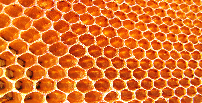
Honeycombs or heaxgonal lattices observed in nature are a popular structure used in composites engineering. Could the same be applied in Additive Manufacturing?
The user needs to customise the behaviour they desire by deriving subclasses from:
These classes serve the purpose for defining a ‘regular’ tessellated sub-region containing hatches. Regular regions that share the same shape characteristics for using the infill optimises the overall clipping performance outlined in the previous post.
Illustration of Checkerboard Island Scan Strategy Implementation
Theoretically, we could build 2D unstructured cells e.g. Voronoi patterns, however, internally hatches for each region will require individual clipping and penalised with a significant performance hit during the hatching process.
Example of a Voronoi diagram: regions are dibi based on the boundaries between.
The Island subclass region is the most important part to re-define the behavior. If we want to change the island regions to become regular tessellated polygons, the localBoundary method should be re-defined. In this example, it will generate a hexagon region, but the implementation below should be generic to cover other N-gon primitives:
   def localBoundary(self) -> np.ndarray:
    # Redefine the local boundary to be the hexagon shape

    if HexIsland._boundary is None:
        # Simple approach is to use a radius to define the overall island size
        #radius = np.sqrt(2*(self._islandWidth*0.5 + self._islandOverlap)**2)

        numPoints = 6

        radius = self._islandWidth / np.cos(np.pi/numPoints)  / 2 + self._islandOverlap

        print('island', radius, self._islandWidth)

        # Generate polygon island
        coords = np.zeros((numPoints+1, 2))

        for i in np.arange(0,numPoints):
            # Subtracting -0.5 orientates the polygon along its face
            angle = (i-0.5)/numPoints*2*np.pi
            coords[i] = [np.cos(angle), np.sin(angle)]

        # Close the polygon
        coords[-1] = coords[0]

        # Scale the polygon
        coords *= radius

        # Assign to the static class attribute
        HexIsland._boundary = coords

    return HexIsland._boundary
The polygon shape is defined by numPoints, so this can be changed to another polygon if desired. The polygon boundary is defined using a radius for the island region and from this a regular polygon is constructed on the outside. The polygon points are rotated by adjusting the start angle so there is a vertical edge on the RHS.
The Polygon is constructed around the island size (radius) and is orientated with the RHS edge vertically
This is generated once as a static class attribute, stored in _boundary to remove the overhead when generating the boundary.
The next step is to generate the internal hatch, which in this occasion needs to be clipped with the local boundary. First, the hatch vectors are generated covering the exterior region using the same radius as the polygon. This ensures that for any rotation transformation of the hatch vectors within the island are fully covered. This is relatively familiar to other code which generates these.
def generateInternalHatch(self, isOdd = True) -> np.ndarray:
    """
    Generates a set of hatches orthogonal to the island's coordinate system :math:`(x\\prime, y\\prime)`.

    :param isOdd: The chosen orientation of the hatching
    :return: (nx3) Set of sorted hatch coordinates
    """

    numPoints = 6

    radius = self._islandWidth / np.cos(np.pi / numPoints) / 2 + self._islandOverlap

    startX = -radius
    startY = -radius

    endX = radius
    endY = radius

    # Generate the basic hatch lines to fill the island region
    x = np.tile(np.arange(startX, endX, self._hatchDistance).reshape(-1, 1), 2).flatten()
    y = np.array([startY, endY])
    y = np.resize(y, x.shape)

    z = np.arange(0, y.shape[0] / 2, 0.5).astype(np.int64)

    coords =  np.hstack([x.reshape(-1, 1),
                            y.reshape(-1, 1),
                            z.reshape(-1,1)])

    # Toggle the hatch angle
    theta_h = np.deg2rad(90.0) if isOdd else np.deg2rad(0.0)

    # Create the 2D rotation matrix with an additional row, column to preserve the hatch order
    c, s = np.cos(theta_h), np.sin(theta_h)
    R = np.array([(c, -s, 0),
                  (s, c, 0),
                  (0, 0, 1.0)])

    # Apply the rotation matrix and translate to bounding box centre
    coords = np.matmul(R, coords.T).T
The next stage is to clip the hatch vectors with the local boundary. This is achieved using the static class method hatching.BaseHatcher.clipLines. The clipped hatches need to be sorted using the ‘z’ index or 2nd column of the clippedLines.
# Clip the hatch fill to the boundary
boundary = [[self.localBoundary()]]
clippedLines = np.array(hatching.BaseHatcher.clipLines(boundary, coords))

# Sort the hatches
clippedLines = clippedLines[:, :, :3]
id = np.argsort(clippedLines[:, 0, 2])
clippedLines = clippedLines[id, :, :]

# Convert to a flat 2D array of hatches and resort the indices
coordsUp = clippedLines.reshape(-1,3)
coordsUp[:,2] = np.arange(0, coordsUp.shape[0] / 2, 0.5).astype(np.int64)
return coordsUp
After sorting, the ‘z’ indexes need to the be condensed or flattened by re-building the ‘z’ index into sequential order. This is done to ensure when the hatches for islands are merged, we simply increment the index of the island using the length of the hatch array rather than performing np.max each time. This is later seen in the method hatching.IslandHatcher.hatch
# Generate the hatches for all the islands
idx = 0
for island in sortedIslands:

    # Generate the hatches for each island subregion
    coords = island.hatch()

    # Note for sorting later the order of the hatch vector is updated based on the sortedIsland
    coords[:, 2] += idx
    ...

    ...
    #
    idx += coords.shape[0] / 2

clippedCoords = np.vstack(clippedCoords)
unclippedCoords = np.vstack(unclippedCoords).reshape(-1,2,3)
HexIslandHatcher
The final stage, is to re-implement hatching.IslandHatcheras a subclass. In this class, at a minimum, the generateIsland method needs to be redefined to correctly positioned the islands so that they tessellate correctly.
def generateIslands(self, paths, hatchAngle: float = 90.0):
    """
    Generate a series of tessellating Hex Islands to fill the region. For now this requires re-implementing because
    the boundaries of the island may be different shapes and require a specific placement in order to correctly
    tessellate within a region.
    """

    # Hatch angle
    theta_h = np.radians(hatchAngle)  # 'rad'

    # Get the bounding box of the boundary
    bbox = self.boundaryBoundingBox(paths)

    print('bounding box bbox', bbox)
    # Expand the bounding box
    bboxCentre = np.mean(bbox.reshape(2, 2), axis=0)

    # Calculates the diagonal length for which is the longest
    diagonal = bbox[2:] - bboxCentre
    bboxRadius = np.sqrt(diagonal.dot(diagonal))

    # Number of sides of the polygon island
    numPoints = 6

    # Construct a square which wraps the radius
    numIslandsX = int(2 * bboxRadius / self._islandWidth) + 1
    numIslandsY = int(2 * bboxRadius / ((self._islandWidth + self._islandOverlap) * np.sin(2*np.pi/numPoints)) )+ 1
The key difference here is defining the number of islands in the y-direction to account for the tessellation of the polygons. This is a simple geometry problem. The y-offset for the islands is simply the vertical component of the 2 x island radius at the angular increment to form the polygon.
Example of tesselation of hexagon islands
The HexIsland are generated with the offsets and appended to the list. These are then treat internally by the parent class IslandHatcher.
...

...

for i in np.arange(0, numIslandsX):
    for j in np.arange(0, numIslandsY):

        # gGenerate the island position
        startX = -bboxRadius + i * self._islandWidth + np.mod(j, 2) * self._islandWidth / 2
        startY = -bboxRadius + j * (self._islandWidth) * np.sin(2*np.pi/numPoints)

        pos = np.array([(startX, startY)])

        # Apply the rotation matrix and translate to bounding box centre
        pos = np.matmul(R, pos.T)
        pos = pos.T + bboxCentre

        # Generate a HexIsland and append to the island
        island = HexIsland(origin=pos, orientation=theta_h,
                            islandWidth=self._islandWidth, islandOverlap=self._islandOverlap,
                            hatchDistance=self._hatchDistance)

        island.posId = (i, j)
        island.id = id
        islands.append(island)

        id += 1

return islands
The island tessellation generated is shown below, with the an offset between islands applied by modifying the radius.
Hexagon Island Boundaries generated across the entire region. The boundaries of the layer are shown, which are used for the intersection test.
The fully clipped scan strategy is shown below with the scanning ordered in the Y-direction.
Hexagonal Island Scan Strategy: Consists of 5 mm Island (radius) with an offset at the boundaries of 0.1 mm.
Conclusions
This post illustrates how one can effectively decompose a layer region into a series of repeatable ‘island’ units which can be processed in an efficient manner, by only clipping hatches at boundary regions. This potentially has the ability to define spatially aware island regions; for example this could be redefining island sizes or parameters towards the boundary of a part. It could be used to alter the scan strategies within the region too, with the effect of changing the thermal behavior.
The hatching performance of PySLM using ClipperLib via PyClipper is reasonably good considering the age of the library using the Vatti polygon clipping algorithm. Without attempting to optimise the underlying library and clipping algorithm for most scenarios, the hatch clipping process should be sufficient for most use case. Future investigation will explore alternative clipping algorithms to further improve the performance of this intensive computational process
For the unfamiliar with the basic hatching process of a single layer, the laser or electron beam (a 1D single point source) must scan across an aerial (2D) region. This is done by creating a series of lines/vectors which infill or raster across the surface.
The most basic form of hatch infill for bulk regions is an alternating, meander, or in some locales referred to a serpentine scan strategy. This tends to be undesirable in SLM due to the creation of localised heat build-up [1] resulting in porosity, poor surface finish [2], residual stress and resultant distortion and anisotropy due to preferential grain growth [3]. Stripe or Island scan strategies are employed in attempt to mitigate these by limiting the length of scan vectors used across a region [4][5][6]. Within the layer hatch vectors for each island are oriented orthogonal to each other and the scan vector length can be precisely controlled in order to reduce the magnitude of residual stresses generated [7].
However, when the user desires a stripe or an island scan strategy, the number of clipping operations for the individual hatch vectors increases drastically. The increase in number of clipping operations increases due to division of the area into fixed size regions corresponding to the desired scan vector length (typically 5 mm)]:
Standard Meander Scan Strategy:n_{clip} \propto \frac{A}{hatchDistance(h_d)}
Island Scan Strategy:n_{clip} \propto \frac{A}{IslandWidth^2}
As can be observed, the performance of hatching with an island scan strategy degrades rapidly when using the island scan due to reciprocal square. As a result, using a naive approach, hatching a very large planar region using an island scan strategy could quickly result in 100,000+ clipping operations for a single layer for a large flat. In addition, this is irrespective of the sparsity of the layer geometry. The way the hatch filling approach works in PySLM, the maximum extent of a contour/polygon region is found. A circle is projected based on this maximum extent, and an outer bounding box is covered. This is explained in a previous post.
The scan vectors are tiled across the region. The reason behind this is to guarantee complete coverage irrespective of the chosen hatch angle, \theta_h, across the layer and largely simplifies the computation. The issue is that many regions will be outside the boundary of the part. Sparse regions both void and solid will not require additional clipping.
The Proposed Technique:
In summary, the proposed technique takes advantage that each island is regular, and therefore each island can be used to discretise the region. This can be used to perform intersection tests for region that may be clipped, whilst recycling existing hatch vectors for those within the interior boundary.
Given that use an island scan strategy provides essentially structured grid, this can be easily transformed into a a method for selecting regions. Using the shapely library, each island boundary consisting of 4 edges can be quickly tested to check if it overlaps internally with the solid part and also intersected with the boundary. This is an efficient operation to perform, despite shapely (libGEOS) being not as efficient as PyClipper.
from shapely.geometry.polygon import LinearRing, Polygon

intersectIslands = []
overlapIslands = []

intersectIslandsSet = set()
overlapIslandsSet= set()

for i in range(len(islands)):

    island = islands[i]
    s = Polygon(LinearRing(island[:-1]))

    if poly.overlaps(s):
        overlapIslandsSet.add(i) # id
        overlapIslands.append(island)

    if poly.intersects(s):
        intersectIslandsSet.add(i)  # id
        intersectIslands.append(island)


# Perform difference between the python sets
unTouchedIslandSet = intersectIslandsSet-overlapIslandsSet
unTouchedIslands = [islands[i] for i in unTouchedIslandSet]
This library is used because the user may re-test the same polygon consecutively, unlike re-building the polygon state in ClipperLib. Ultimately, this presents three unique cases:
Non-Intersecting (shapely.polygon.intersects(island) == False) – The Island resides outside of the boundary and is discarded,
Intersecting (shapely.polygon.intersects(island) == True) – The Island is in an internal region, but may be also clipped by the boundary,
Clipped (shapely.polygon.intersects(island) == True) – The island intersects with the boundary and requires clipping.
The result is shown here for a simple 200 mm square filled with 5 mm islands:
Taking the difference between cases 2) and 3), the islands with hatch scan vectors can be generated without requiring unnecessary clipping of the interior scan vectors. As a result this significantly reduces the computational effort required.
Although extreme, the previous example generated a total number of 2209 5 mm islands to cover the entire region. The breakdown of the island intersections are:
Non-intersecting islands: 1591 (72%),
Non-clipped islands: 419 (19%),
Clipped islands: 199 (9%).
With respect to solid regions, the number of clipped islands account for 32% of the total area. The overall result is shown below. The total area of the hatch region that was hatched is 1.97 \times 10^3 \ mm^2, which is equivalent to a square length of 445 mm, significantly larger than what is capable on most commercial SLM systems. Using an island size of 5 mm with an 80 μm hatch spacing, the approximate hatching time is 6.5 s on a modest laptop system. For this example, 780 000 hatch vectors were generated.
A close up view showing the 5mm Island Hatching with 0.8 mm Hatch Distance. Blue Lines show the overall path traversed by the laser beam. The total time taken for hatching was approximately 8 seconds.
The order of hatching scanned is shown by the blue lines, which trace the midpoints of the vectors. Hatches inside the island are scanned sequentially. The order of scanning in this case is chosen to go vertically upwards and then horizontally across using the in-built Python 3 sorting function with a lambdaexpression Remarkably, all performed using one line:
A future post will elaborate further methods for sorting hatch vectors and island groups.
Comparison to Original Implementation:
The following is a non-scientific benchmark performed to illustrate the performance profile of the proposed method in PySLM.
Island Size [mm]
Original Method Time [s]
Proposed Method Time [s]
3
466
5.3
5
258
6.5
10
121
7.9
20
75
8.23
Approximate benchmark comparing Island Hatching Techniques in PySLM
It is clearly evident that the proposed method reduces the overall time by 1-2 orders for hatching a region. What is strange is that with the new proposed method, the overall time increases with the island size.
Generally it is expected that the number of clipping operations n_{clip} to be the following:
n_{clip} \propto \frac{Perimiter}{IslandWidth}
Potentially, this allows bespoke complex ‘sub-island’ scan strategies to be employed without a significant additional cost because scan vectors within un-clipped island regions can be very quickly replicated across the layer.
Other Benefits
The other benefits of taking approach is making a more modular object orientated approach for generating island based strategies, which don’t arbitrarily follow regular structured patterns. A future article will illustrate further explain the procedures for generating these.
Parry, L. A., Ashcroft, I. A., & Wildman, R. D. (2019). Geometrical effects on residual stress in selective laser melting. Additive Manufacturing, 25. https://doi.org/10.1016/j.addma.2018.09.026
Valente, E. H., Gundlach, C., Christiansen, T. L., & Somers, M. A. J. (2019). Effect of scanning strategy during selective laser melting on surface topography, porosity, and microstructure of additively manufactured Ti-6Al-4V. Applied Sciences (Switzerland), 9(24). https://doi.org/10.3390/app9245554
Zhang, W., Tong, M., & Harrison, N. M. (2020). Scanning strategies effect on temperature, residual stress and deformation by multi-laser beam powder bed fusion manufacturing. Additive Manufacturing, 36(June), 101507. https://doi.org/10.1016/j.addma.2020.101507
Ali, H., Ghadbeigi, H., & Mumtaz, K. (2018). Effect of scanning strategies on residual stress and mechanical properties of Selective Laser Melted Ti6Al4V. Materials Science and Engineering A, 712(October 2017), 175–187. https://doi.org/10.1016/j.msea.2017.11.103
Robinson, J., Ashton, I., Fox, P., Jones, E., & Sutcliffe, C. (2018). Determination of the effect of scan strategy on residual stress in laser powder bed fusion additive manufacturing. Additive Manufacturing, 23(February), 13–24. https://doi.org/10.1016/j.addma.2018.07.001
This quantity is arguably the greatest driver of individual part cost for the majority of Additive Manufacture parts (excluding the additional costs of post-processing). It inherently relates to the proportional utilisation of the AM system that has a fixed capital cost at purchase under an assumed operation time (estimate is around 6-10 years).
Predicting this quickly and effectively for parts built using Powder Bed Fusion processes may initially sound simple, but actually there aren’t many free or opensource tools that provide a utility to predict this. Also the data isn’t not easily obtainable without having some inputs. In the literature, investigations into build-time estimation, embodied energy consumption and the analysis of costs associated with powder-bed for both SLM and EBM have been undertaken [1][2][3][4].
This usually involves submitting your design to an online portal or building up a spreadsheet and calculating some values. A large part of the cost for a part designed for AM is related to its build-time and this as a value can indicate the relative cost of the AM part.
Build-time, as a ‘lump’ measure is quintessentially the most significant factor in determining the ultimate cost of parts manufactured on powder-bed fusion systems. Obviously, this is oblivious to other factors such as post-processing of parts (i.e. heat-treatment, post-machining) surface coatings and post-inspection and part level qualification, usually essentially as part of the entire manufacturing processes for an AM part.
The reference to a ‘lump’ cost value coincides with various parameters inherent to the part that are driven by the decisions of design to meet the functional requirements / performance. The primary factors affecting this:
Material alloy
Geometrical shape of the part
Machine system
These may be further specified as a set of chosen parameters
Part Orientation
Build Volume Packing (i.e. number of parts within the build)
Number of laser beams in the SLM system
Recoater time
Material Alloy laser [arameters (i.e. effective laser scan speed)
Part Volume (V)
From the build-time, the cost estimate solely for building the piece part can be calculated across ‘batches’ or a number of builds, which largely takes into account fixed costs such as capital investment in the machine and those direct costs associated with material inputs, consumables and energy consumption [5].
In this post, additional factors intrinsic to the machine operation, such as build-chamber warm-up and cool-down time, out-gassing time are ignored. Exploring the economics of the process, these should be accounted for because it can in some processes e.g. Selective Laser Sintering (SLS) and High-Speed-Sintering (HSS) of polymers can account for a significant contribution to the actual ‘accumulated‘ build time within the machine.
Calculation of the Build Time in L-PBF
There are many different approaches for calculating the estimate of the build-time depending on the accuracy required.
Build Bulk Volume Method
The build volume method is the most crudest forms for calculating the build time, t_{build}. The method takes the total volume of the part(s) within a build V and divided by machine’s build volume rate \dot{V} – a lumped empirical value corresponding to a specific material deposited or manufactured by an AM system.
t_{build}=\frac{V}{\dot{V}}
This is very approximate, therefore limited, because the prediction ignores build height within the chamber that is a primary contributor to the build time. Also it ignores build volume packaging – the density of numerous parts contained packed inside a chamber, which for each build contributes a fixed cost. However, it is a good measure for accounting the cost of the part based simply on its mass – potentially a useful indicator early during the design conceptualisation phase.
Layer-wise Method
This approach accounts for the actual geometry of the part as part of the estimation. It performs slicing of the part and accounts for the area and boundaries of the part, which may be assigned separate laser scan speeds. This has been implemented as a multi-threaded/process example in order to demonstrate how one can analysis the cost of a part relatively quickly and simply using this as a template.
The entire part is sliced at the constant layer thickness L_t in the function calculateLayer(). In this function, the part is sliced using getVectorSlice(), at the particular z-height and by disabling returnCoordPaths parameter will return a list of Shapely.geometry.Polygon objects.
The slice represents boundaries across the layer. Each boundary is a Shapely.Polygon, which can be easily queried for its boundary length and area. This is performed later after the python multi-processing map call:
d = Manager().dict()
d['part'] = solidPart
d['layerThickness'] = layerThickness

# Rather than give the z position, we give a z index to calculate the z from.
numLayers = int(solidPart.boundingBox[5] / layerThickness)
z = np.arange(0, numLayers).tolist()

# The layer id and manager shared dict are zipped into a list of tuple pairs
processList = list(zip([d] * len(z), z))

startTime = time.time()

layers = p.map(calculateLayer, processList)
p.close()
print('multiprocessing time', time.time()-startTime)

polys = []
for layer in layers:
    for poly in layer:
        polys.append(poly)

layers = polys

"""
Calculate total layer statistics:
"""
totalHeight = solidPart.boundingBox[5]
totalVolume = solidPart.volume

totalPerimeter = np.sum([layer.length for layer in layers]) * numCountourOffsets
totalArea = np.sum([layer.area for layer in layers])
Once the sum of the total part area and perimeter are calculated the total scan time can be calculated from these. The approximate measure of scan time across the part volume (bulk region) is related by the total scan area accumulated across each layer of the partA, the hatch distance h_d and the laser scan speed v_{bulk}.
t_{hatch} = \frac{A}{L_t v_{bulk}}
Similarly the scan time across the boundary for contour scans (typically scanned at a lower speed is simply the total perimeter length L divided by the contour scan speed v_{contour}
t_{boundary} = \frac{L}{v_{contour}}
Finally, the re-coating time is simply a multiple of the number of layers.
In fact, it may be possible to deduce that much of this is unnecessary for finding the approximate scanning time. Instead, a simpler formulation can be derived. The scan time can be deduced from simply the volume Vand the total surface area of the part S
where N=h_{build}/L_t. After realising this, further looking into literature, it was proposed by Giannatsis et al. back in 2001 for SLA time estimation [6]. Surprisingly, I haven’t come across this before. They propose that taking the vertical projection of the surface better represents the true area of the boundary, under the slicing process.
The projected area is calculated by taking the dot product with the vertical vector v_{up} = (0.,0.,1.0)^T and the surface normal \hat{n} using the relation: a\cdot b = \|a\| \|b\| \cos(\theta) for each triangle and calculating the sine component using the identity (\cos^2(\theta) + \sin^2(\theta) = 1) to project the triangle area across the vertical extent.
Comparison between build time estimation approaches
The difference in scan time with the approximation is relatively close for a simple example:
Discretised Layer Scan Time – 4.996 hr
Approximate Scan Time – 5.126 hr
Approximate Scan Time (with projection) – 4.996 hr
Arriving at the rather simple result may not be interesting, but given the frequency of most cost models not stating this hopefully may be useful for some. It is useful in that it can account for the complexity of the boundary rather than simply the volume and the build-height, whilst factoring in the laser parameters used – typically available for most materials on commercial systems .
The second part of the posting will share more details about more precisely measuring the scan time using the analysis tools available in PySLM.
Baumers, M., Tuck, C., Wildman, R., Ashcroft, I., & Hague, R. (2017). Shape Complexity and Process Energy Consumption in Electron Beam Melting: A Case of Something for Nothing in Additive Manufacturing? Journal of Industrial Ecology, 21(S1), S157–S167. https://doi.org/10.1111/jiec.12397
Baumers, M., Dickens, P., Tuck, C., & Hague, R. (2016). The cost of additive manufacturing: Machine productivity, economies of scale and technology-push. Technological Forecasting and Social Change, 102, 193–201. https://doi.org/10.1016/j.techfore.2015.02.015
Faludi, J., Baumers, M., Maskery, I., & Hague, R. (2017). Environmental Impacts of Selective Laser Melting: Do Printer, Powder, Or Power Dominate? Journal of Industrial Ecology, 21(S1), S144–S156. https://doi.org/10.1111/jiec.12528
Liu, Z. Y., Li, C., Fang, X. Y., & Guo, Y. B. (2018). Energy Consumption in Additive Manufacturing of Metal Parts. Procedia Manufacturing, 26, 834–845. https://doi.org/10.1016/j.promfg.2018.07.104
Giannatsis, J., Dedoussis, V., & Laios, L. (2001). A study of the build-time estimation problem for Stereolithography systems. Robotics and Computer-Integrated Manufacturing, 17(4), 295–304. https://doi.org/10.1016/S0736-5845(01)00007-2
Much of slicing and hatching process is already taken for granted in commercial software mostly offered by the OEMs of these systems rarely discussed amongst academic research. Already we observe practically the implications direct control over laser parameters and scan strategy on the quality of the bulk material – reduction in defects, minimising distortion due to residual stress, and the surface quality of parts manufactured using these process. Additionally, it can have a profound impact the the metallic phase generation, micro-structural texture driven via physics-informed models [1], grading of the bulk properties and offer precise control over manufacturing intricate features such as thin-wall or lattice structures [2].
This post hopefully highlights to those unfamiliar some of the basis process encountered in the generation of machine build files used in AM systems and get a better understanding to the operation behind PySLM. I have tried my best to generalise this as much as possible, but I imagine there are subtleties I have not come across.
This post is to provide some reference into the generation of hatches or scan vectors are created for use in AM processes such as selective laser melting (SLM), which uses a point energy source to raster across a medium. Some people prefer to more generally to classify the family of processes using the technical ASTM F42 committee standards 52900 and 52911 – Powder Bed Fusion (PBF). I won’t go into the basic process of the manufacturing processes such as EBM, SLM, SLA, BJF, as there are many excellent articles already that explain these in far greater detail.
Machine Build Files
AM processes require a digital representation to manufacture an object. These tend to be computed offline – separate from the 3D Printer, using specialist or dedicated pre-processing software. I expect this will become a closed-loop system in the future, such that the manufacturing integrated directly into the machine.
For some AM process families, the control operations may be exceedingly granular – i.e. G-code. G-code formats state specific instructions or functional commands for the 3D printer to sequentially or linearly execute. These tend to fit with deposition methods such as Filament Extrusion, Direct-Ink-Writing (robo-casting) and direct energy deposition (DED) methods. Typically, these tends to be for deposition with a machine systems, which requires coordination of physical motion in-conjunction with some mechanised actuation to deposit/fuse material.
Machine Build File Formats for L-PBF
For exposure (laser, electron-beam) based AM processes, commercial systems use a compact notation solely for representing the scan path the exposure source will traverse . The formats are often binary to aid their compactness.
To summarise, within these build files, an intermediate representation consists of index-based referenceable parameters for the build. The remainder consists of a series of layers, that contain geometric entities (points, vectors) that are used to to control the exposure for the border or contour or raster or infill the interior region. For L-PBF processes, the digital files, commonly referred as “machine build file” comes in various flavours dependent on the machine manufacture:
Renshaw .mtt,
SLM Solution .slm,
DMG Mori Realizer .rea
EOS .sli
Aconity .cli+ or .ilt wrapper
Some file formats, such as Open Beam Path format can specify bezier curves [3]. Another recently proposed open source format created by RWTH Aachen in 2022 called OpenVector Format based on Google’s Protobuf schema. The format aims to offer a specification universally compatible across a swathe of PBF processes and supplement existing commercial formats with additional build-process meta-data (e.g. build, platform temperature, dosing) and detailed definition with further advancements in the process, such as multi-beam builds.
Build-File Formats
Higher level representations that describe the distribution of material(s) defining geometry – this could be bitmap slices or even a 3D model. Processes such as Jetting, BJF, High Speed Sintering, DLP Vat-polymerisation currently available offer this a reality. With time, polymer and metal processes will evolve to become 2D:, diode aerial melting [4] or more aerial based scanning based on holographic additive manufacturing methods, such as those proposed by Seurat AM [5] based off research at LLNL, and recently at University of Cambridge [6] . In the future, we can already observe the exciting prospect of new processes such as computed axial lithograph [7] that will provide us near instantaneous volumetric additive manufacturing.
For now, single and multi point exposure systems for the imminent future will remain with us as the currently available process. PySLM uses an intermediate representation – specifying a set of points and lines to control the exposure of energy into a layer.
The Slicing and Hatching Process in L-PBF
With nearly most conventional 3D printing process, it begins with a 3D representation of a solid volume or geometry. 2D planar slices or layers are extracted from a 3D mesh or B-Rep surface in CAD by taking cross-sections from a geometry. Each slice layer consist of a set of boundaries and holes describing the cross-section of an object. Note: non-planar deposition does exist for DED/Filament processes, such as this Curved Layer Fused Deposition Modeling [ref] and a spherical slicing technique [8].
For consolidating material, an exposure beam must raster across the surface medium (metal or polymer powder, or a photo-polymer resin) depending on the process. Currently this is a single or multiple point which moves at a velocity vwith a power P across the surface. The designated exposure or energy deposited into the medium is principally a function of these two parameters, depending on the type of laser:
(Quasi)-Continious Wave: The laser remains active switched on (typically modulated using a form of PWM) across the entire length of the scan vector
Pulsed Mode (Q-Switched): Laser is pulsed at set distances and exposure times across the scan vector
Numerous experiments often tend to result in parametric power/speed maps to the achieved part bulk density, that result in usually optimal processing windows that produce stable and consistent melt-tracks [9][10]. Recently, process maps are based on a non-dimensional parameter such as the normalised enthalpy approach, that more reliably assist selecting a suitable process windows [11].
However, the complexity of the process extends further and is related to a many additional variables dependent on the process such as layer thickness, absorption coefficient (powder and material), exposure beam profile etc.. Additionally, the cumulative energy deposited spatially over a period of time must consider overlap of scan vectors within an area.
Scan Vector Generation
Each boundary polygon is offset initially to account for the the radius of the beam exposure, which is termed a ‘spot compensation factor‘. Some processes such as SLS or BJF account for global part shrinkage volumetrically throughout the part by having a global scale factor or deformed mesh to compensate to non-uniform shrinkage across the part.
The typical composition of a layer used for scanning in exposure based processes. This consists of outer and inner contours, with the core interior filled with hatches.
This first initial offset is the outer-contour which would be visible on the exterior of the part. This contour will have a different set of laser parameters in order to optimise and improve the surface roughness of the part obtained. A further offset is applied to generate a set of inner-contours before hatching begins.
Depending on the orientation of the surface (e.g. up-skinor down-skin), the boundary and interior region may be intersected to fine-tune the laser parameters to provide better surface texture, or surface roughness – typically varying between Ra = 3-13 μm [12] primarily determined by the surface angle and a combination of the process variables including,
the powder feedstock (bulk material, powder size distribution)
laser parameters
layer thickness (pre-dominantly fixed or constant for most AM processes)
Overhang regions and surfaces with a low overhang angles tend to be susceptible to high surface-roughness. Roller re-coater L-PBF systems – available only on 3DSystems or AddUp system,, tend to offer far superior surface quality on low inclined or overhang regions. Additionally, progressive advancement and maturity of laser parameter optimisation, and those computationally driven using part geometry [13] are able to further enhance the quality and potentially eliminate the need for support structures. Depending on the machine platform, these regions are identified by sampling across two-three layers. Overhang regions obviously require support geometry, which is an entirely different topic discussed in this post.
Laser parameters can be optimised based on the adjacent surface regions. Special regions, include the upskin, downskin and overhang regions needed to improve the surface roughness and reduce density in regions.
Following the generation of the contours, the innercore region requires filling with hatches. Hatches are a series of parallel scan vectors placed adjacent at a set hatch distance, h_d. This parameter is optimized according to the material processed, but is essentially related to the spot radius of the exposure point r_s in order to reduce inter-track and inter layer porosity. Across each layer these tend to be placed at a particular orientation \theta_h, which is is then incrementally rotated globally for subsequent layers, typically 66.6°. This rotation aims to smooth out the build process in order to minimise inter-track porosity, and generate homogeneous material, and in the case of SLM mitigate the effects of anisotropic residual stress generation.
A general composition of the various LayerGeometry objects used to scan across a Layer. The various parameters such as the hatch distance, spacing and hatch angle are shown.
The distribution (position, length, rotation) of these hatch vectors are arranged using a laser scan strategy. The most common include a simple alternating hatch, stripe and island or checkerboard scan strategy.
Each set or group of scan vectors is stored together in a LayerGeometry, depending on the type (either a set of point exposures, contour or hatch vectors). These LayerGeometry groups usually share a set of exposure parameters – power, laser scan speed (point exposure time, point distance for a pulsed laser), focus position).
Some systems offer a greater degree of control and can control individual power across the scan vectors. Other can fine tune the acceleration and modulate the power along the scan vectors to support techniques known as ‘skywriting‘. For instance in SLM, it has been proposed that careful tuning of the laser parameters towards the end of the scan vector, i.e. turning can reduce porosity by preventing premature collapse of key holing phenomena [14]. In theory, PySLM could be extended to provide greater control of the electro-optic systems used in the process if so desired.
Hopefully, this provides enough background for those who are interested and engaged in working with developing scan strategies and material development using PySLM.
Plotkowski, A., Ferguson, J., Stump, B., Halsey, W., Paquit, V., Joslin, C., Babu, S. S., Marquez Rossy, A., Kirka, M. M., & Dehoff, R. R. (2021). A stochastic scan strategy for grain structure control in complex geometries using electron beam powder bed fusion. Additive Manufacturing, 46. https://doi.org/10.1016/j.addma.2021.102092
Ghouse, S., Babu, S., van Arkel, R. J., Nai, K., Hooper, P. A., & Jeffers, J. R. T. (2017). The influence of laser parameters and scanning strategies on the mechanical properties of a stochastic porous material. Materials and Design, 131, 498–508. https://doi.org/10.1016/j.matdes.2017.06.041
Zavala Arredondo, Miguel Angel (2017) Diode Area Melting Use of High Power Diode Lasers in Additive Manufacturing of Metallic Components. PhD thesis, University of Sheffield.
Kelly, B., Bhattacharya, I., Shusteff, M., Panas, R. M., Taylor, H. K., & Spadaccini, C. M. (2017). Computed Axial Lithography (CAL): Toward Single Step 3D Printing of Arbitrary Geometries. Retrieved from http://arxiv.org/abs/1705.05893
Yigit, I. E., & Lazoglu, I. (2020). Spherical slicing method and its application on robotic additive manufacturing. Progress in Additive Manufacturing, 5(4), 387–394. https://doi.org/10.1007/s40964-020-00135-5
Yadroitsev, I., & Smurov, I. (2010). Selective laser melting technology: From the single laser melted track stability to 3D parts of complex shape. Physics Procedia, 5(Part 2), 551–560. https://doi.org/10.1016/j.phpro.2010.08.083
Maamoun, A. H., Xue, Y. F., Elbestawi, M. A., & Veldhuis, S. C. (2018). Effect of selective laser melting process parameters on the quality of al alloy parts: Powder characterization, density, surface roughness, and dimensional accuracy. Materials, 11(12). https://doi.org/10.3390/ma11122343
Ferro, P., Meneghello, R., Savio, G., & Berto, F. (2020). A modified volumetric energy density–based approach for porosity assessment in additive manufacturing process design. International Journal of Advanced Manufacturing Technology, 110(7–8), 1911–1921. https://doi.org/10.1007/s00170-020-05949-9
Ni, C., Shi, Y., & Liu, J. (2019). Effects of inclination angle on surface roughness and corrosion properties of selective laser melted 316L stainless steel. Materials Research Express, 6(3). https://doi.org/10.1088/2053-1591/aaf2d3
Martin, A. A., Calta, N. P., Khairallah, S. A., Wang, J., Depond, P. J., Fong, A. Y., … Matthews, M. J. (2019). Dynamics of pore formation during laser powder bed fusion additive manufacturing. Nature Communications, 10(1), 1–10. https://doi.org/10.1038/s41467-019-10009-2