After a long period, PySLM version 0.6 is released. This coincides with the intensity of commitments as a new academic at the University of Nottingham over the past year. The release has mainly focused on improvements and enhancements to the underlying codebase rather than the addition of entirely new features. There are several substantial changes to the underlying dependencies that contributes some improvements and performance throughout which PySLM users will benefit from.
Dependency changes
With the release of ClipperLib2 library, additional python bindings were exposed and released as a separate library in the PyClipr. These were created using the PyBind11 headers and provides the core functionality required to performing offsetting and clipping of path segments and hatch vectors. There are no substantial feature improvements inherited from the change, but a noticeable performance improvement can be observed. Another benefit is that PySLM does not require compilation via cython and is now a full source distribution available via PyPi repositories.
Another significant dependency change is the use of the manifold mesh Boolean library. This offers a substantial improvement to mesh manipulation operations, that are fundamental to successful support generation for use in metal L-PBF. The library provides robust intersection of water-tight meshes, that is also computationally efficient when compared to the prior PyClipr library which was based on the clipr library from over a decade ago. This significantly improves the quality of the volumes generated in BlockSupportBase and those derived from these such as those with the GridTrussSupport that provide perforations and teeth for metal L-PBF. Additionally, this removes an additional dependency that requires maintenance by myself, and is more cross-platform that what can be offered by the previous PyClipr library.
Further incremental changes, that will not affect users is migration to the Shapely 2.0 library and also Trimesh 4.0, which required some internal changes to maintain compatibility.
Support Generation Improvements:
The support generation has been improved to be more robust and reliable compared to the initial release in version 0.5.0. Further robustness checks are implemented in the ray-tracing method developed in version 0.5, for identifying correctly the support projection height maps which are used to identify boundaries of the support volume. Further use has been explored in applied research by TWI – see open access paper (An Interactive Web-Based Platform for Support Generation and Optimisation for Metal Laser Powder Bed Fusion) by Dimopoulos et al.
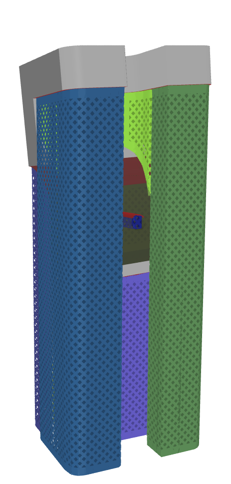
By default all BlockSupport‘s have smoothed boundaries by the use of spline fitting, which was previously only applied on self-intersecting supports. Smooth boundaries significantly improve the quality of the final GridBlockSupport, because the perforated grid truss skin can more smoothly conform to the boundary of the support volume.
Smoothed boundaries generated for all SupportVolumes for a complex part: including both self-intersecting supports and those only connected to the build-plate
As a recommendation to users, care must be taken to not smoothen the boundaries too much or these will not correctly conform to the original geometry causing the ray-projection algorithm to fail. A recommending starting point for the spline simplification factor is between 5-30, but is dependent on the relative part scale. Coinciding with the use of the manifold3d library, there is an appreciable improvement in the speed for generating the support volumes.
Another improvement is the more configurable parameters for Grid Truss Support generation. This includes further enhancement and control over the perforated teeth, across both upper and lower support volume surfaces. These are fully customisable by a user function, which ensure that a repeating shape is conformed in 3D across the surface profiles of the support volume.
Finally, a significant enhancement is correctly pre-sorting the scan vectors within the sliced support regions to take advantage of the line segments when scanning by the beam source. This significantly improves build productivity by minimising jumps across adjacent segments and ensures that the galvo-mirror movement remains mostly in the same direction.
A layer showing the order of scanning across all grid truss support generated for a complex topology optimised part. Jump distance is a total of 2056 mm with a total scan vector length 1377 mm.
Documentation Improvements
Further improvements to the inline documentation have been included alongside improvements and examples that are now provided on readthedocs. These provide basic information and guides for using PySLM, some of which is consolidated from these blog entries to aid new users using the library. Over time these will be further enhanced and amended to support researchers and users wishing to use PySLM in their work.
Conclusions & Change Log
The release has taken a while to release, but overall has received a level of polish and refinement that helps the release find use amongst more in commercially vested R&D projects and academic research. There are other developments still in the pipeline but much focus was on providing a long-term stable release for users. The full changelog can be found here.
Pyclipr is a Python library offering the functionality of the Clipper2 polygon clipping and offsetting library and are built upon pybind . The underlying Clipper2 library performs intersection, union, difference and XOR boolean operations on both simple and complex polygons and also performs offsetting of polygons and inflation of un-connected paths. Unfortunately, the contracted name (Clipr) is the closest name to that of the previous form.
Unlike pyclipper, this library is not built using cython, which was previously integrated directly into PySLM with custom modifications to provide ordering of scan vector. Instead the full capability of the pybind binding library is exploited, which offers great flexibility and control over defining data-structures. This library aims to provide convenient access to the modifications and new functionality offered by Clipper2 library for Python users, especially with its usage prevalent across most open source 3D Printing packages (i.e. Cure) and other computer graphics applications.
Summary of key ClipperLib2 Features Relevant to AM and their use in PySLM
Improved performance and numerical robustness
Simplification of open-path clipping – no requirement to use PolyPath usage
Built-in numerical scaling between floating point and the internal Int64
Additional point attributes built-in directly (Z-attribute)
Summary of Implementation
The structure follows closely with ClipperLib2 api in most cases but has adapted some of the naming to be more pythonic and regularity during typing.
The added benefit of the original PyClipper library is that it can take numpy and native python lists directly, because these are implicitly converted by pybind into the internal vector format. A significant addition is the ability to accept 2D paths with the additional ‘Z’ attributes (currently floating points) without using separate functions, taking advantage of pythons duck typing. Open-paths and these optionally defined z attributes are returned when passing the arguments when performing the execute function for clipping utilities. Below are a summary of the key operations
Path Offsetting
Path offsetting is accomplished relatively straightforwardly. Paths are added to the ClipperOffset object and the join and end types are set. The delta or offset distance is then provided in the execute function.
import numpy as np
import pyclipr

# Tuple definition of a path
path = [(0.0, 0.), (0, 105.1234), (100, 105.1234), (100, 0), (0, 0)]
path2 = [(0, 0), (0, 50), (100, 50), (100, 0), (0,0)]

# Create an offsetting object
po = pyclipr.ClipperOffset()

# Set the scale factor to convert to internal integer representation
pc.scaleFactor = int(1000)

# add the path - ensuring to use Polygon for the endType argument
po.addPath(np.array(path), pyclipr.Miter, pyclipr.Polygon)

# Apply the offsetting operation using a delta.
offsetSquare = po.execute(10.0)
Polygon Intersection
Polygon intersection can be perform by using the Clipper object. This requires add individual path or paths and then setting these as subject and clip. The execute call is used and can return multiple outputs depending on the clipping operation. This includes open-paths or Z attribute information.
# continued

# Create a clipping object
pc = pyclipr.Clipper()
pc.scaleFactor = int(1000) # Scale factor is the precision offered by the native Clipperlib2 libraries

# Add the paths to the clipping object. Ensure the subject and clip arguments are set to differentiate
# the paths during the Boolean operation. The final argument specifies if the path is
# open.

pc.addPaths(offsetSquare, pyclipr.Subject)
pc.addPath(np.array(path2), pyclipr.Clip)

""" Polygon Clipping """
# Below returns paths of various clipping modes
outIntersect  = pc.execute(pyclipr.Intersection)
outUnion = pc.execute(pyclipr.Union)
outDifference = pc.execute(pyclipr.Difference, pyclipr.EvenOdd) # Polygon ordering can be set in the final argument
outXor = pc.execute(pyclipr.Xor, pyclipr.EvenOdd)

# Using execute2 returns a PolyTree structure that provides hierarchical information
# if the paths are interior or exterior

outPoly = pc.execute2(pyclipr.Intersection, pyclipr.EvenOdd)
Open Path Clipping
Open-path clipping (e.g. line segments) may be performed natively within pyclipr, by default this is disabled. Within the execute function, returnOpenPaths argument should be set true.
""" Open Path Clipping """
# Pyclipr can be used for clipping open paths.  This remains simple to complete using the Clipper2 library

pc = pyclipr.Clipper()
pc2.scaleFactor = int(1e5)

# The open path is added as a subject (note the final argument is set to True to indicate Open Path)
pc2.addPath( ((50,-10),(50,110)), pyclipr.Subject, True)

# The clipping object is usually set to the Polygon
pc2.addPaths(offsetSquare, pyclipr.Clip, False)

""" Test the return types for open path clipping with option enabled"""
# The returnOpenPaths argument is set to True to return the open paths. Note this function only works
# well using the Boolean intersection option

outC = pc2.execute(pyclipr.Intersection, pyclipr.NonZero)
outC2, openPathsC = pc2.execute(pyclipr.Intersection, pyclipr.NonZero, returnOpenPaths=True)
Z-Attributes
The final script of note is the in-built Z attributes that are embedded within PyClipr. Z attributes (float64) can be attached to each point across a path or. set of polygons. During intersection of segments or edges, these Z attributes are passed to the resultant clipped paths. These are returned as a separate list in the output.
""" Test Open Path Clipping """

pc3 = pyclipr.Clipper()
pc3.scaleFactor = int(1e6)

pc3.addPath(openPathPolyClipper, pyclipr.Clip, False)

# Add the hatch lines (note these are open-paths)
pc3.addPath( ((50.0,-20, 3.0),
              (50.0 ,150,3.0)), pyclipr.Subject, True) # Open path with z-attribute of 3 at each path point

""" Test the return types for open path clipping with different options selected """
hatchClip = pc3.execute(pyclipr.Intersection, pyclipr.EvenOdd, returnOpenPaths=True)

# Clip but return with the associated z-attributes
hatchClipWithZ = pc3.execute(pyclipr.Intersection, pyclipr.EvenOdd, returnOpenPaths=True, returnZ=True)
Usage in PySLM
PyClipr has been refactored for use in the next release of PySLM (v0.6). This has improved readability of code and in some cases there are performance improvements due to inherent optimisations within ClipperLib2. This includes also removal of unnecessary transformations and scaling factors performed within python, that were required converting between paths generated in PySLM (shapely) and PyClipper originally. In particular, avoiding the use of PolyNodes were especially useful to avoid throughout. Modifications have been applied throughout the entire modules including the hatching and support modules. PySLM also now benefits by becoming a purely a source distribution, by distribution the clipping and offsetting functions into a separate package, therefore no additional compiling is required during installation.
The default mesh slicing option available in PySLM, Part.getVectorSlice was never particularly aimed at being high throughput at the beginning. It aimed to simply offer the functionality to test hatching approaches, that utilised existing approaches available within Trimesh. The built-in slicing option built-upon using trimesh.intersections.mesh_plane functionality existing already and was used for this purpose. This slicing option has been robust, and the author has considered edge-cases that may occur during the intersection between the slicing plane and triangular meshes. This includes additionally shell and to a limited extent processing non-manifold meshes. Additionally, an arbitrary choice of slicing plane may be used, which for 3D graphics is useful, however, for 3D printing, typically nearly all processes work layer-wise in the Z direction.
In the Trimesh implementation, a few optimisation have been built-in. When slicing multiple planes across a mesh using trimesh.intersections.mesh_multiplane, the dot product is pre-calculated between the mesh vertices and the plane normal and origin may be cached and re-used for subsequent computations across multiple slices.
Existing Accelerated Slicing Approaches
Despite the relative time spent during slicing is likely less than the majority of spent within the final hatching process that fills the part with hatch vectors. Nevertheless, the performance wasn’t adequate especially for larger triangular meshes. Some direct approaches could have been low-level optimisation using specialised Python libraries (e.g. Numba, Pyston) or re-coding in underlying c++ code. A better approach was considered.
Building-upon a recent research paper by Minetto et al. [1] , it is possible to improve the performance by selectively pre-sorting and filter triangles of the mesh the to reduce the overall complexity to O(n+m+k), where n is the number of triangles, m is the number of slices and k is the number of intersections. Their method determines the coverage each triangle and separates these to an individual list of triangles for each slice layer to isolate potential intersections in order to reduce the search space size. Inadvertently, the slicing operation becomes trivially parallel to process.
The second focus on their paper is using hash structure to more efficiently combine the generated line segments/paths from the slicing operation into correctly orientated paths. This process ensures a consistent winding number for clipping operations later. Their approach relies on rounding the coordinates within a tolerance, to identify coincident points. However, is reliant on water-tight meshes. Another author applies a variation, however, uses Graph instead of a Hash table with a modest improvement [2]. Curiously, I noticed a big discrepancy between their reported performance. For PySLM, the polygon construction is internally handled automatically using the ClipperLib or Shapely polygon processing libraries.
The key thing taken from that paper and previous research was that by pre-sorting the triangle mesh based on predefined ‘constant’ layer thickness, potential intersecting triangle candidates within the mesh can be extracting during the computation and interestingly parallelised.
Methodology
Provided mesh, the approach first extracts the minimum and maximum Z positions per triangle, which correspond with the bottom and top most layer that a potential mesh intersection occurs. This corresponds to Algorithm 2 in the previous cited paper. Across the generated list of layer slices, a binary search (numpy.searchsorted) across a pre-sorted list is used for identifying these locations. Across each triangle, their array index is appended to each layer within an inefficient for loop. Overall, the cost of this pre-sorting is only expensive when assembling the indices across the layer. Afterwards, these may then be used during the slicing stage.
# Generate a list of slices for each layer across the entire mesh
zSlices = np.linspace(-5, 5, 200)
k = 1000 # number of slices
zMin, zMax = myMesh.bounds[:,2]
zBox = np.linspace(zMin, zMax, k)


tris = myMesh.triangles

# Obtain the min and maximum Z values across the entire mesh
zVals = tris[:, :, 2]
triMin = np.min(zVals, axis=1)
triMax = np.max(zVals, axis=1)


# Below is a manual approach to sorting and collecting the triangles across each layer

if False:

    triSortIdx = np.argsort(triMinMax[1,:])
    triMinMaxSort = triMinMax[:,triSortIdx]

    startTime = time.time()

    sortTris = []

    iSects2 = []
    for i in range(len(zBox)):
        minInside = zBox[i].reshape(-1,1) > triMinMax[0, :].reshape(1, -1)
        maxInside = zBox[i].reshape(-1,1) < triMinMax[1, :].reshape(1, -1)
        iSects2.append(np.argwhere((minInside & maxInside).ravel()))

    print('endTime array base', time.time() - startTime)

# An alteratnvie more compact way is to use binary search operator available within
# numpy.searchsorted. This locates the bottom and top layer position

minIdx = np.searchsorted(zBox, triMin, side='left')
maxIdx = np.searchsorted(zBox, triMax, side='left')

# Attach the corresponding presorted triangles into the
iSects = [[] for i in range(len(zBox))]

# The iterative part for assigning potential triangles for intersection on a triangle are performed here
# Note: Process is very inefficient in native Python O(n*k)
for i in range(len(minIdx)):

    startLayer = minIdx[i]
    endLayer = maxIdx[i]
    for layer in iSects[startLayer:endLayer+1]:
        layer.append(i)
Plane-Triangle Intersections
The pre-processing has been completed, now the final slincg may be complete. Performing some micro-optimisations, further refactoring may be done to adapt the code previously present in Trimesh.
The process of slicing or intersection, is simple. Suprisingly, there are a no obvious references for this process. Slicing a triangular mesh, relies firstly computing the potential intersection of each edge of a faceted mesh, in this case it is generalised for an abritrary plane. Firstly, the vector between the mesh vertices (v_i) and the plane origin (v_o) is calculated – red lines in the diagram. The dot product is taken with the slicing plane normal \textbf{n}. The sign of the dot product indicates if the point lies above or below the plane – zero uniquely is the intersection.
This is extremely convenient to compute, and it only requires the calculation of the Z component because X,Y components are typically zero for planar or layer-wise 3D printing. This becomes a trivial solution, the sign of the difference between the Z position and plane indicates if it is above or below a plane.
For the simplest case: when the signs are opposite across a triangular edge indicates that one point lies above the plane, and the other below. This reduces the number of further operations required. The actual points for intersection across the edge, is simply the linear interpolation of the vector along the edge based on the Z distance between the mesh and the points on the edge.
This can be achieve from the following
t = plane_origin[2] - endpoints[0,:,2]
b = line_dir[:, 2]
d = np.divide(t, b)
intersection = endpoints[0]
intersection = intersection + np.reshape(d, (-1, 1)) * line_dir
Using the pre-sorted triangles from earlier, the indices can be use to extract triangle information to calculate the potential opportunities each triangle intersection may intersect. In the original Trimesh function intersection.mesh_plane, this can be done by using the local_faces and the cache_dot arguments:
For small meshes, this is likely to have a performance penalty for sorting and grouping of triangles. Nevertheless, for large meshes this should provide a substantial improvement because of the likelihood achieving drastic reduction in the potential number of intersection planes within the mesh. Due to independent separation of triangles within the mesh corresponding to a series of slice planes, this is trivially parallelisable as the journal articles conclude. Further optimisations were performed on the trimesh routines to increase the performance a little further.
Numba Optimisation
For further performance improvements, the intersection code in Trimesh mesh_plane was re-programmed using numba. Numba uses the LLVM compiler to JIT recompilation and convert native python bytecode re-interpretation into an intermediate representation that can be further optimised for the target architecture (CPU/GPU) that includes fine-tuning for optional multi-core processing. Additionally, some internal functions are optimised and Furthermore, type introspection is performed automatically to maxis performance.
Numba is easy to use for transforming existing code with minimal effort for prototyping purposes and has direct equivalents for numpy functions. Existing code can be translated by including the appropriate numba imports (jit, njit, prange) and prepending function (kernels) with the appropriate numba function decorator @njit. Multi-processing can be triggered with an additional argument in the @njit function decorator and fine-grained control with the use of prange. An example used on a binary search function, provided below:
from numba import njit, prange

@njit(parallel=False)
def searchsorted_parallel(a, b):
    res = np.empty(len(b), np.intp)
    for i in prange(len(b)):
        res[i] = np.searchsorted(a, b[i])
    return res
From experience, parallel performance in the particular use case offered little advantage. Another observation is that the use of single precision (float32) compared to the default double precision (float64) type offers negligible performance gains at least on an ARM64 architecture.
Note the implementation described in the post ignores sequential sorting of the generated line segments into correctly orientated connected paths that can construct polygons.
Benchmarking
The optimised slicing approach was applied on a double gyroid lattice structure that was subdivided consisting of 6.3 million triangles, with triangle intersections evenly distributed across the volume (k=10 800 ± 1090). The slicing was performed across 1000 individual slices, with the reported slicing time (extracting un-ordered segments) that was measured with the various approaches tried, that are currently used in PySLM:
The above approaches were based on a single processor/core using Python 3.8, and the performance was evaluated across 7 runs using %timeit in the ipython console and the results are presented on the side. Unlike the default implementation in PySLM, these do not generated ordered polygons via the shapely library.
It can be observed that there is a improvement in the slicing performance by ordering and grouping of intersected triangles.
Benchmarking the slicing performance using three approaches on a gyroid matrix mesh (6.3 million triangles)
Conclusions
The approach implemented is relatively simple to introduce and can be built already on existing functionality provided by trimesh. The post does not intend to infer that Trimesh’s slicing functionality is insufficient, rather, by building upon existing functionality it can enhance its performance substantially. This is even without requiring programming optimisation offered by numba. Further work is potentially needed to optimise the creation of ordered connecting paths, this may investigated further.
The functionality will be incorporated into a dedicated slicer class in a future upcoming release of PySLM.
Minetto, R., Volpato, N., Stolfi, J., Gregori, R. M. M. H., & da Silva, M. V. G. (2017). An optimal algorithm for 3D triangle mesh slicing. Computer-Aided Design, 92, 1–10. https://doi.org/10.1016/j.cad.2017.07.001
The in-built visualisation for scan paths in PySLM leverages matplotlib – refer to a previous post. This is sufficient for most user’s needs when attempting to interpret and visualise the scan paths generated in PySLM, or those imported from a slice taken from an existing machine build files. Extending this beyond multiple layers or large parts becomes more tricky when factoring in visualisation of some parameters (e.g. Laser Power, effective scan speed). Admittedly, the performance of Matplotlib becomes limited to explore the intricacies and complexities embedded within the scan vectors.
For scientific research, the fusion of scan vector geometry with volumetric datasets such as X-Ray CT during post-inspection of parts/samples, or those generated within the build process including pyrometry data, thermal-imaging offer the ability to increase our understanding and insight to observations of the effect of process on the material produced using L-PBF. GPU based visualisation libraries such (vispy) would offer the possibility to accelerate the performance, but are not user-friendly nor offer interactivity when manipulating views and the data and are often cumbersome when processing volumetric datasets often encountered in Additive Manufacturing. Paraview is a cross-platform open-source scientific visualisation tool that is especially powerful for processing, interaction and visualisation of large-scale scientific datasets.
Paraview and the underlying VTK library offers an alternative ready-made solution to visualise this information, and are most importantly hardware accelerated with the option for raytracing provided by OSPRay and OptiX for latest RTX NVIDIA cards that include Raytracing (RT) cores. Additionally, the data can be augmented and processed using parallelised filters and tools in Paraview.
VTK File Format
Ignoring the HDF5 variations that are most useful for structured data, the underlying format within vtk that used for storing vector based data and point cloud data is the .vtp file format. The modern VTK file formats use an XML schema – unlike the legacy format, to store a structured series of geometry (volumetric data, lines, polygons, 3D elements and point clouds). The internal data format can be stored using ascii encoding or binary. Binary data can be incorporated directly within a parsable .xml format using a Base64 encoding and may additional incorporate internal compression. Alternatively data can be stored in an appended data section located at the footer of the file, which treats data section as a contiguous block of raw data. Different sub-formats exist, that are appropriate for different types of data e.g. volumetric, element based (Finite Volume / Finite Element derived) or polygon based. An approach relevant to export scan vector geometry the .vtp – format is most suitable.
The data stored in the VTK Point file consists of:
3D points coordinates
Data attributes stored at each point location
Geometric elements (lines, polygons) defining connectivity with reference to the list of point coordinates
Paraview exporter implementation:
The Paraview exporter is simplistic, because the data compression is currently ignored. The process is similar to the technique used in the function pyslm.visualise.plotSequential, whereby hatch and contour vectors are merged and reprocessed in order that they represent always a series of lines (an n x 2 x 2 array). This is not the most efficient option for ContourGeometry (border scans) where scan vectors are continuously joined up, but simplifies the processing working with the data.
Once the scan vector coordinates and the relevant data are packaged up into a single array, the data is wrote within the sub-sections of the XML file. Data is stored using floating points or integers accordingly in a binary representation. The data used to represent coordinates and indices for each vector, are stored with the ‘appended’ option within the <DataArray> element of each section. The raw data is stored and collected that are then written in the <AppendedData> element at the end of file with raw encoding option chosen. The byte offsets for the position of each ‘chunk’ of data that are referenced by the <DataArray> element are collected and stored incrementally.
For reference, the following information is provided for writing raw data, because this was difficult to obtain from the VTK documentation directly.
<AppendedData encoding=”raw”>
Start of Raw Data Section
_
Underscore character is starting location for reading raw data
Section Size (Int32/Int64)
Integer representing size of following section (include the size in bytes with the offsets provided). The integer type should match the size used in the header.
Raw data (e.g Int32, float32, float64)
….
Repeated the above (two rows) for each referenced data section
</AppendedData>
Example Scan Vector Data exported to VTK
An example Aconity .ILT file was imported into PySLM and then exported to a .vtp VTK file that was processed in Paraview. The scan order is visualised by the colour map with each vertex assigned a global-id. The ‘Tube‘ filter was applied to each scan vector in order to improve their visibility.
The script excerpt can currently be found on a Gist. This will be later included in future versions of PySLM along with other import/exporters.
Digital Light Projector (DLP) 3D Printers are an exceptionally productive technique for producing highly detailed (30<𝝁m) parts at high speeds at minimal costs.The CLIP process is a further enhancement in build speeds.
Briefly, the DLP process is similar to Stereolithography (SLA). It cures a vat of UV curable polymer material above a flexible transparent PTFE membrane. Instead of a single exposure (UV laser) into the resin, a monochrome LCD screen is used to mask the UV exposure source underneath. A greyscale bitmap image is used for each layer. Typically for most systems, after exposing the layer (1.5-3 s), the upper build-platform retracts, and mechanically pulls the cured layer away from the flexible membrane and the process is repeated. Surprisingly simple, but effective in cost and the production speed.
Additionally, bitmap based approaches are used amongst Material Jetting (MJ) technologies predominantly used within our research group CfAM, at Nottingham. Both DLP and Material Jetting offer high resolution between 30-100 𝝁m both in the XY slice plane dependent on the printer, and for Inkjet downwards of 1-10 𝝁m layer thickness depending on the choice of ink loading. Accordingly, these high resolutions are demanding to print. I came accustomed to using these printers in our CfAM lab at Nottingham on a recent project. The affordability of these printers is genuinely remarkable, owing to their mechanical simplicity.
Based on a previous post back in 2016 by Dr Matt Keeter, this is an excellent reference to an approach using WebGL implementation. Their post introduced the method, but the approach was obscured by its WebGL based implementation. Frutstratingly, I never came across an implementation for use in a research environment. These appraoches are most likely used in the free slicer software provided for desktop DLP 3D Printers.
Anycubic Mono 4k DLP Printer at the University of Nottingham’s CfAM Lab loaded with a composite ink. 2022.
Interestingly, this approach can also be extended for generating 3D voxel models, by applying the project across multiple directions. However, the reliability of such method for non-manifold meshes would likely be limiting.
Method for Bitmap Slicing
The method is similar and use the same infrastructure to that used in the previous post for performing height map ray projection. Likewise, to provide a cross-platform compatibility, the use of Vispy and OpenGL 2.0 GLSL shaders are utilised within a single script. As such, the resolution of the output is limited to the maximum framebuffer size supported by the GPU driver on the system.
The approach for generating slices relies on having a connected watertight with surface triangles normals correctly orientated (fixable natively using Trimesh). The approach uses a combination of Stencil buffers integrated natively in GPU hardware.
By choosing an appropriate Z-clipping plane for the camera, the Stencil buffer is used to keep and discard rasterised triangles with the z-clipping range based on the Z-order. In order to determine if the fragments rendered are inside or outside the mesh. The render pipeline uses three passes:
Pass 1: stencil buffer increments on front facing fragments
Pass 2: stencil buffer decrements on back facing fragments
Pass 3: discard fragments where the stencil buffer is zero
During all the render passes, GL Depth tests are turned off. Typically in 3D Programs, triangles that are obscured from view of the 3D camera, or hidden behind other triangles are culled and the fragment is discarded prior to rendering . In this method, depth testing is turned off. The full approach is detailed further in the excerpt below inside the on_draw call.
def on_draw(self, event):

    with self._fbo:
        # Set the GL state
        gloo.set_state(blend=False, stencil_test=True, depth_test=False, polygon_offset_fill=False, cull_face=False)

        # Set the size of the framebuffer to fit the geometry with the correct aspect ratio
        gloo.set_viewport(0, 0, self._visSize[0], self._visSize[1])
        gloo.set_clear_stencil(0)
        gloo.set_clear_color((0.0, 0.0, 0.0, 0.0))

        # Clear the framebuffer
        gloo.clear()

        self.program['bounds'] = self.bbox[0,2], self.bbox[1,2]
        self.program['aspect'] = self.physical_size[1] /  self.physical_size[0]

        # The position of the slice position passed to the GLSL shader
        self.program['frac'] = self._z * 2.0

        # Draw twice, adding and subtracting values in the stencil buffer

        # Render Pass 1 (Increment Stencil Buffers)
        gloo.set_stencil_func('always', 0, 0xff)
        gloo.set_stencil_op('keep', 'keep', 'incr', 'back')
        gloo.set_stencil_op('keep', 'keep', 'keep', 'front')
        self.program.draw('triangles', self.filled_buf)

        # Render Pass 2 (Decrease Stencil Buffers)
        gloo.set_stencil_op('keep', 'keep', 'decr', 'front')
        gloo.set_stencil_op('keep', 'keep', 'keep', 'back')
        self.program.draw('triangles', self.filled_buf)

        # Clear only the color buffer
        gloo.clear(color=True, depth=False, stencil=False)

        # Render Pass 3
        gloo.set_stencil_func('notequal', 0, 0xff)
        gloo.set_stencil_op('keep', 'keep', 'keep')
        self.program.draw('triangles', self.filled_buf)

        # Store the final framebuffer
        self.rgb = _screenshot((0, 0, self._visSize[0], self._visSize[1]))
The GLSL shaders are not particularly interesting. Focus should be given to the Vertex shader, rather than the Fragment shader. This Vertex shader processes vertices of the mesh and applies the Model View Projection (MVP) transformation matrix onto the input mesh. The MVP matrix is chosen to scale the entire geometry so that it fits within the Z-clipping range of Z = -1 to +1, and is within the scope of rendering into Stencil buffer whilst using the 3D Orthographic Camera. Finally, the model is transformed based on a fractional range (0-1) to obtain the required Z-slicing plane. An epsilon value is provided for round-off purposes.
uniform   mat4 u_model; // Model transform matrix
uniform   mat4 u_view;
uniform   mat4 u_projection;

uniform  vec2 bounds; // Z bounds
uniform  float frac;  // Z fraction (0 to 1)
uniform  float aspect; // Aspect ratio

attribute vec3 a_position;

#define EPSILON 0.001

void main() {

    vec3 pos = a_position;

    // Ensure the bottom of the part is positioned to z=0 using the bottom bounding box
    pos.z -= bounds[0];

    // Scale the so that it fits within the clipping range (-1.0 < z < 1.0)
    pos.z *= -2.0/(bounds[1]-bounds[0]);

    // Adjust the position of  the verticies
    pos.z -= frac;
    gl_Position = u_projection * u_view * u_model * vec4(pos, 1.0);
    gl_Position.z += 1.0 - EPSILON;
}
The remainder of the script sets up the infrastructure for Vispy. This is performed within the initialisation call for the script. This methods sets up the correct OpenGL state, viewport size including the use of an off-screen render and specific selection of a separate Stencil framebuffer used to render onto. Both the vertex and fragment shaders are compiled and the transformation matrix is generated based on an Orthographic projection sized to the bounding box of the geometry.
    # Window Size
    shape = int(self._visSize[1]), int(self._visSize[0])

    # Create the render texture used by default in the pipeline
    self._rendertex = gloo.Texture2D((shape + (4,)), format='rgba', internalformat='rgba32f')

    # These are not used but are for reference
    #self._colorBuffer = gloo.RenderBuffer(self.shape, format='color')
    #self._depthRenderBuffer = gloo.RenderBuffer(shape, format='depth')

    # Create the stencil buffer (8 bit component)
    self._stencilRenderBuffer = gloo.RenderBuffer(shape, format='stencil')
    self._stencilRenderBuffer.resize(shape, format=gloo.gl.GL_STENCIL_INDEX8)

    # Create FBO, attach the color buffer and depth buffer
    self._fbo = gloo.FrameBuffer(self._rendertex)
    self._fbo.stencil_buffer=self._stencilRenderBuffer

    # Set the size of the view port based on the size of the window (the bounding box)
    gloo.set_viewport(0, 0, self.physical_size[0], self.physical_size[1])
    gloo.set_viewport(0, 0, self._visSize[0], self._visSize[1])

    # Create the initial orthographic view projection transformation based on the bounding box of the geometry
    self.projection = ortho(self.bbox[1, 0], self.bbox[0, 0], self.bbox[1, 1], self.bbox[0, 1], 2, 40)
    # Identity matrix
    self.model = np.eye(4, dtype=np.float32)

     # Set MVP variables for shaders
    self.program['u_projection'] = self.projection
    self.program['u_model'] = self.model
    self.program['u_view'] = self.view
Other operations are processing and the Trimesh and correctly transformed into the correct position:
The script was applied to a porous aerofoil structure with an XY resolution of 20 µm that was used previously on an Anycubic DLP system. Below is an example cross-section taken using this approach. Notice the high resolution
Conclusions
The overall approach may have a limited use by itself. Generally, the need to bespoke high resolution slices are limited at this stage. For reference, the full excerpt of the script is temporarily located here. In future, I will consider including this as another option within PySLM.
In the past, I have used Paraview for visualising voxel models and finite element meshes. Paraview is geared towards scientific visualisation built towards ray-tracing capability for volumes and meshes using OSPRay. Unfortunately, despite options to automate their preparation of models using packages such as PyVista, it often required additional manual image editing. I wanted to find an alternative that semi-automates some of the model visualisation and also improve the quality of the visualisation, whilst providing some additional ‘glossy’ pictures for this website.
Mitsuba 3, is a cross-platform open source photorealistic render originating Wenzel Jakob. This alongside some other photo-realistic rendering codes that are available and can operate within Python. For most purposes these codes are targeted for `academi’c education and for research use for developing accurate physical light rendering models. Some academic papers have used this also for rendering their 3D mode with a better aesthetic quality compared to mainstream mesh editing programs or visualisation software.
Mitsuba is straightforward to setup and install within a standard Python environment (pip install Mitsuba). Mitsuba’s documentation is reasonable to follow in terms of documentation of their plugins and API, however, the number of examples and python excerpts was a little lacking beyond those packaged bundled ‘scene.xml’ files.
For reference, below is an excerpt that can be used to assist with rendering some objects. This involves creating a scene definition using a Python Dict object. Be aware that additional ‘realistic’ material BSDF models are available, such as metal, plastic and transparent/translucent materials. The scene is relatively simple, consisting of a circular disc (z=0) to cast shadows upon to. Careful seleciton of light emitters (area lights) should be provide good illumination in the scene, otherwise convergence and noise artefacts can become present in the render. Crucially, in this script the mesh provided is rescaled and positioned above the disc plane based on the Z-height.
Note: an average of the bounding box could be taken. This is done in order to simplfify the alignment and position of the perspective camera in the scene and make it independent of the geometry provided.
import os
import numpy as np
import matplotlib.pyplot as plt
import mitsuba as mi
from mitsuba import ScalarTransform4f as T

import trimesh
from trimesh.transformations import rotation_matrix

mi.set_variant('scalar_rgb')

# Load the mesh file here
myMesh = trimesh.load('bracket.stl')

# Scale the mesh to approximately one unit based on the height
sf = 1.
myMesh.apply_scale(sf/myMesh.extents[2])
myMesh = myMesh.apply_transform(rotation_matrix(np.deg2rad(90), [1.0,0.0,0]))

# Translate the mesh so that it's centroid is at the origin and rests on the ground plane
myMesh.apply_translation([-myMesh.bounds[0,0] - myMesh.extents[0] / 2.0,
                          -myMesh.bounds[0,1] - myMesh.extents[1] / 2.0,
                          -myMesh.bounds[0,2]])

# Fix the mesh normals for the mesh
myMesh.fix_normals()

# Write the mesh to an external file (Wavefront .obj)
with open('mesh.obj', 'w') as f:
    f.write(trimesh.exchange.export.export_obj(myMesh,include_normals=True ))

#Create a sensor that is used for rendering the scene
def load_sensor(r, phi, theta):
    # Apply two rotations to convert from spherical coordinates to world 3D coordinates.
    origin = T.rotate([0, 0, 1], phi).rotate([0, 1, 0], theta) @ mi.ScalarPoint3f([0, 0, r])

    return mi.load_dict({
        'type': 'perspective',
        'fov': 40.0,
        'to_world': T.look_at(
            origin=origin,
            target=[0, 0, myMesh.extents[2]/2],
            up=[0, 0, 1]
        ),
        'sampler': {
            'type': 'independent',
            'sample_count': 16
        },
        'film': {
            'type': 'hdrfilm',
            'width': 1024,
            'height': 768,
            'rfilter': {
                'type': 'tent',
            },
            'pixel_format': 'rgb',
        },
    })

# Scene parameters
relativeLightHeight = 5.0

# A scene dictionary contains the description of the rendering scene.
scene2 = mi.load_dict({
    'type': 'scene',
    # The keys below correspond to object IDs and can be chosen arbitrarily
    'integrator': {'type': 'path'},

    'mesh': {
        'type': 'obj',
        'filename': 'mesh.obj',
        'face_normals': True, # This prevents smoothing of sharp-corners by discarding surface-normals. Useful for engineering CAD.
        'bsdf': {
            'type': 'diffuse',
            'reflectance': {
                'type': 'rgb',
                'value': [0.1, 0.27, 0.86]
            }
        }
    },

    # A general emitter is used for illuminating the entire scene (renders the background white)
    'light': {'type': 'constant', 'radiance': 1.0},
    'areaLight': {
        'type': 'rectangle',
        # The height of the light can be adjusted below
        'to_world': T.translate([0,0.0,myMesh.bounds[1,2] + relativeLightHeight]).scale(1.0).rotate([1,0,0], 5.0),
        'flip_normals': True,
        'emitter': {
            'type': 'area',
            'radiance': {
                'type': 'spectrum',
                'value': 25.0,
            }
        }
    },

    'floor': {
        'type': 'disk',
        'to_world': T.scale(3).translate([0.0,0.0,0.0]),
        'material': {
            'type': 'diffuse',
            'reflectance': {'type': 'rgb', 'value': 0.75},
        }
    }
})

sensor_count = 1

radius = 8
phis = [70.0]
theta = 60.0

sensors = [load_sensor(radius, phi, theta) for phi in phis]

"""
Render the Scene
The render samples are specified in spp
"""
image = mi.render(scene2, sensor=sensors[0], spp=256)

# Write the output
mi.util.write_bitmap("my_first_render.png", image)
mi.util.write_bitmap("my_first_render.exr", image)

# Display the output in an Image
plt.imshow(image** (1.0 / 2.2))
plt.axis('off')
A sample output is produced below of topology optimised bracket used with the above script. In the scene a flat disc (Z=0) is illuminated by a global ‘constant’ light emitter and an area emitter to provide soft shadows.
Render of a topology optimised bracket using the Mitsuba 3 Renderer.
On a laptop, this took approximately 30s to render a 1024×768 to 128 samples per pixel (SPP). Renders are relatively quick to generate on modern multi-core computer systems using just their CPUS.
Rendering Meshes with Vertex Colours
Plotting just geometry in a single colour isn’t very interesting, especially when we have results or extra data stored within the mesh. Mitsuba has the option to render colours assigned to each vertex.These can be extracted relatively easily from Finite Element meshes, or other functions. This normally would be trivial, but a subtle trick required is adapting the script to export to the .ply format and separately assign the vertex colour attribute within the scene structure. This can be done by setting the option within the BSDF diffuse material reflectance property, as documented
Trimesh, to date, exports 4-component (RGBA) vertex-colour attribute to the .ply format. The 4-component vertex-colour attribute, however, is unfortunately incompatible with Mitsuba, therefore the data array must be attached separately to the loaded scene, using the traverse function. This can be done by accessing the ‘mesh’ object within the declared Mitsuba scene.
Note:Mitusba uses DrJit for its data representation, but this directly interoperates with numpy arrays. For updating the internal buffer data in the scene, a flat data structure must be supplied to the vertex attribute property.
myMitsubaMesh = scene2.shapes()[2] # Access the .ply mesh object in the loaded scene
# Add a separate 3 component vertex colour attribute with the same number of vertices as the mesh
myMitsubaMesh.add_attribute('vertex_color', 3, [0] * myMesh.vertices.shape[0])
N = myMesh.vertices.shape[0]
# Use Mitsuba traverse function to modify data in the scene graph/structure
meshParams = mi.traverse(myMitsubaMesh)
# Generate a colour mapping based solely on the z-corrdiante of the mesh
vertColor = trimesh.visual.color.interpolate(myMesh.vertices[:,2], 'Paired') [:,:3] / 255.0
# Update the vertex colour data buffer/array in mitsuba associated with the .ply mesh
meshParams["vertex_color"] = vertColor.ravel()
meshParams.update()
The full example excerpt is presented below
import os
import numpy as np
import mitsuba as mi
import matplotlib.pyplot as plt
import drjit as dr
mi.set_variant('scalar_rgb')
from mitsuba import ScalarTransform4f as T
import trimesh
from trimesh.transformations import rotation_matrix
# Load the mesh file here
myMesh = trimesh.load('bracket.stl')
# Scale the mesh to approximately one unit based on the height
sf = 1.
myMesh.apply_scale(sf/myMesh.extents[2])
myMesh = myMesh.apply_transform(rotation_matrix(np.deg2rad(90), [1.0,0.0,0]))
# Translate the mesh so that it's centroid is at the origin and rests on the ground plane
myMesh.apply_translation([-myMesh.bounds[0,0] - myMesh.extents[0] / 2.0,
-myMesh.bounds[0,1] - myMesh.extents[1] / 2.0,
-myMesh.bounds[0,2]])
# Fix the mesh normals for the mesh
myMesh.fix_normals()
# Write the mesh to an external file (Wavefront .obj)
with open('mesh.ply', 'wb') as f:
f.write(trimesh.exchange.export.export_ply(myMesh))
#Create a sensor that is used for rendering the scene
def load_sensor(r, phi, theta):
# Apply two rotations to convert from spherical coordinates to world 3D coordinates.
origin = T.rotate([0, 0, 1], phi).rotate([0, 1, 0], theta) @ mi.ScalarPoint3f([0, 0, r])
return mi.load_dict({
'type': 'perspective',
'fov': 40.0,
'to_world': T.look_at(
origin=origin,
target=[0, 0, myMesh.extents[2]/2],
up=[0, 0, 1]
),
'sampler': {
'type': 'independent',
'sample_count': 16
},
'film': {
'type': 'hdrfilm',
'width': 1024,
'height': 768,
'rfilter': {
'type': 'tent',
},
'pixel_format': 'rgb',
},
})
# Scene parameters
relativeLightHeight = 5.0
# A scene dictionary contains the description of the rendering scene.
scene2 = mi.load_dict({
'type': 'scene',
# The keys below correspond to object IDs and can be chosen arbitrarily
'integrator': {'type': 'path'},
'mesh': {
'type': 'ply',
'filename': 'mesh.ply',
'face_normals': True,
'bsdf': {
    'type': 'diffuse',
    'reflectance': {
        'type': 'mesh_attribute',
        'name': 'vertex_color'
    }
}
},
# A general emitter is used for illuminating the entire scene (renders the background white)
'light': {'type': 'constant', 'radiance': 1.0},
'areaLight': {
'type': 'rectangle',
# The height of the light can be adjusted below
'to_world': T.translate([0,0.0,myMesh.bounds[1,2] + relativeLightHeight]).scale(1.0).rotate([1,0,0], 5),
'flip_normals': True,
'emitter': {
'type': 'area',
'radiance': {
'type': 'spectrum',
'value': 25.0,
}
}
},
'floor': {
'type': 'disk',
'to_world': T.scale(3).translate([0.0,0.0,0.0]),
'material': {
'type': 'diffuse',
'reflectance': {'type': 'rgb', 'value': 0.75},
}
}
})
myMitsubaMesh = scene2.shapes()[2]
myMitsubaMesh.add_attribute('vertex_color', 3, [0] * myMesh.vertices.shape[0])
N = myMesh.vertices.shape[0]
#vertex_colors = dr.zeros(mi.Float, 3 * N)
#vertex_colors +=
#vertex_colors /= 255
meshParams = mi.traverse(myMitsubaMesh)
vertColor = trimesh.visual.color.interpolate(myMesh.vertices[:,2], 'Paired') [:,:3] / 255.0 #paired / plasma
meshParams["vertex_color"] = vertColor.ravel()
meshParams.update()
sensor_count = 1
radius = 8
phis = [70.0]
theta = 60.0
sensors = [load_sensor(radius, phi, theta) for phi in phis]
"""
Render the Scene
The render samples are specified in spp
"""
image = mi.render(scene2, sensor=sensors[0], spp=256)
# Write the output
mi.util.write_bitmap("my_first_render.png", image)
mi.util.write_bitmap("my_first_render.exr", image)
plt.imshow(image** (1.0 / 2.2))
plt.axis('off')
The output of this is shown below, which uses a stratified colour map to render the z-value position. On closer inspect it can be observed that the interpolation of the Z position is interpolated across each triangle, so the precise isolevel boundaries are not exact. For most purposes, using a high resolution mesh, this would not cause concern.
Rendering of a topology optimised bracket with Z component isolevels generated and attached as vertex_color attribute
Rendering Volumetric Textures
Mitusba 3, provides the opportunity to both render volumes and interestingly apply volumes interpolated as volumetric surface textures. In this situation, a 3-component (RGB) voxel grid can be generated and intersecting values corresponding with intersecting mesh surface are used as the colour information.
Render of a topology optimised bracket with a volume field attached as a surface texture
Mitsuba uses its own simple .vol format for storing voxel grid information, although a convenient Python function does not exist for this. The definition of the current file format used is presented in the table. This is relatively simple to generate and export using Python’s inbuilt file handing functions. More efficient approaches would simply write the Numpy array directly to the file by correctly ordering the data in the array with the channel data (last axis) moving the fastest across the flattened array.
Position [Bytes]
Content
1-3
ASCII Bytes ’V’, ’O’, and ’L’
4
File format version number (currently 3)
5-8
Encoding identified (32-bit integer). 1 = Float32
9-12
Number of cells along the X axis (32 bit integer)
13-16
Number of cells along the Y axis (32 bit integer)
17-20
Number of cells along the Z axis (32 bit integer)
21-24
Number of channels (32 bit integer, supported values: 1, 3 or 6)
25-48
Axis-aligned bounding box of the data stored in single precision (order: xmin, ymin, zmin, xmax, ymax, zmax)
49-*
Binary data of the volume stored in the specified encoding. The data are ordered so that the following C-style indexing operation makes sense after the file has been loaded into memory: data[((zpos*yres + ypos)*xres +xpos)*channels + chan] where (xpos, ypos, zpos, chan) denotes the lookup location.
Structure of the .vol file format used by Mitsuba (version 3.0)
Below is an excerpt of the function that can export a numpy 4D (m \times n \times p \times 3 ) array with three colour channels to this file format.
def writeVol(filename, vol: np.ndarray, bbox):

    def int8(val) -> bytes:
        return struct.pack('b', val)

    def int32(val) -> bytes:
        return struct.pack('i', val)

    def float(val) -> bytes:
        return struct.pack('f', val)

    with open(filename, 'wb') as f:
        f.write('VOL'.encode('ascii'))
        f.write(int8(3))
        f.write(int32(1)) # 1 = float type
        f.write(int32(vol.shape[0]) ) # X grid size
        f.write(int32(vol.shape[1]))  # Y grid size
        f.write(int32(vol.shape[2]))  # Z grid size

        f.write(int32(vol.shape[3])) # Number of channels

        # Write the bounding Box of the grid
        # Values [x0,y0,z0, x1,y1,z1]

        f.write(bbox.astype(np.float32).tobytes())

        for k in range(vol.shape[2]):
            for j in range(vol.shape[1]):
                for i in range(vol.shape[0]):
                    for m in range(vol.shape[3]):
                        f.write(float(vol[i,j,k,m]))
An excerpt is presented below for generating a TPMS lattice U field. A volume is generated with an equal number of unit cells across each dimension covering the bounding box of the mesh. The values of the U field are transformed using matplotlib colourmap via trimesh.visual.color.interpolate as before and these are exported as the Mitsuba volume format using the inline function writeVol() . Later in the scene definition, this is transformed to align with the original mesh by using the ‘to_world‘ attribute
import os
import numpy as np
import mitsuba as mi
import drjit as dr
import struct
mi.set_variant('scalar_rgb')

from mitsuba import ScalarTransform4f as T

import matplotlib.pyplot as plt

import trimesh
from trimesh.transformations import rotation_matrix

def writeVol(filename, vol: np.ndarray, bbox):

    def int8(val) -> bytes:
        return struct.pack('b', val)

    def int32(val) -> bytes:
        return struct.pack('i', val)

    def float(val) -> bytes:
        return struct.pack('f', val)

    vol.shape[0]

    with open(filename, 'wb') as f:
        f.write('VOL'.encode('ascii'))
        f.write(int8(3))
        f.write(int32(1)) # 1 = float type
        f.write(int32(vol.shape[0]) ) # X grid size
        f.write(int32(vol.shape[1]))  # Y grid size
        f.write(int32(vol.shape[2]))  # Z grid size

        f.write(int32(vol.shape[3])) # Number of channels

        # Write the bounding Box of the grid
        # Values [x0,y0,z0, x1,y1,z1]
        print('bounding box', bbox)
        f.write(bbox.astype(np.float32).tobytes())

        for k in range(vol.shape[2]):
            for j in range(vol.shape[1]):
                for i in range(vol.shape[0]):
                    for m in range(vol.shape[3]):
                        f.write(float(vol[i,j,k,m]))


# Load the mesh file here
myMesh = trimesh.load('bracket.stl')
myMesh = myMesh.apply_transform(rotation_matrix(np.deg2rad(90), [1.0,0.0,0]))
#myMesh.apply_scale([2.5,1,3.0])

# Resolution of the Lattice Grid (note if this is set too low, Mitsuba has render issues)...
res = 0.3499

# Create a gyroid field
Lx = myMesh.extents[0]
Ly = myMesh.extents[1]
Lz = myMesh.extents[2]

""" Number of lattice unit cells"""
cellLength = 5.0

kx = Lx/cellLength
ky = Ly/cellLength
kz = Lz/cellLength

""" Create the computational grid - note np operates with k(z) numerical indexing unlike the default matlab equivalent"""
x,y,z = np.meshgrid(np.arange(0.0, Lx, res),
                    np.arange(0.0, Ly, res),
                    np.arange(0.0, Lz, res))


"""
Calculating the Gyroid TPMS
"""
Tg = 0.7

U = ( np.cos(kx*2*np.pi*(x/Lx))*np.sin(ky*2*np.pi*(y/Ly))
    + np.cos(ky*2*np.pi*(y/Ly))*np.sin(kz*2*np.pi*(z/Lz))
    + np.cos(kz*2*np.pi*(z/Lz))*np.sin(kx*2*np.pi*(x/Lx)) )**2 - Tg**2

vol = trimesh.visual.color.interpolate(U, 'plasma').reshape(list(U.shape) + [4])[:,:,:,:3] / 256.0

# Delete the temporary variables
del x,y,z, U

# Scale the mesh to approximately one unit based on the height
sf = 2.5
myMesh.apply_scale(sf/myMesh.extents[2])

# Translate the mesh so that it's centroid is at the origin and rests on the ground plane
myMesh.apply_translation([-myMesh.bounds[0,0] - myMesh.extents[0] / 2.0,
                          -myMesh.bounds[0,1] - myMesh.extents[1] / 2.0,
                          -myMesh.bounds[0,2]])


# Fix the mesh normals for the mesh
myMesh.fix_normals()

# Write the volume
bounds = myMesh.bounds.reshape(-1,1).copy()
bounds = np.array([0,0,0,1,1,1])

# Write out the volume
writeVol('out.vol', vol, bounds)


# Write the mesh to an external file (Wavefront .obj)
with open('mesh.ply', 'wb') as f:
    f.write(trimesh.exchange.export.export_ply(myMesh))

#Create a sensor that is used for rendering the scene
def load_sensor(r, phi, theta):
    # Apply two rotations to convert from spherical coordinates to world 3D coordinates.
    origin = T.rotate([0, 0, 1], phi).rotate([0, 1, 0], theta) @ mi.ScalarPoint3f([0, 0, r])

    return mi.load_dict({
        'type': 'perspective',
        'fov': 40.0,
        'to_world': T.look_at(
            origin=origin,
            target=[0, 0, myMesh.extents[2]/2],
            up=[0, 0, 1]
        ),
        'sampler': {
            'type': 'independent',
            'sample_count': 30,

        },
        'film': {
            'type': 'hdrfilm',
            'width': 1024,
            'height': 768,

            'pixel_format': 'rgb',
        },
    })

# Scene parameters
relativeLightHeight = 5.0

# A scene dictionary contains the description of the rendering scene.
scene2 = mi.load_dict({
    'type': 'scene',
    # The keys below correspond to object IDs and can be chosen arbitrarily
    'integrator': {'type': 'path'},


    'mesh': {
        'type': 'ply',
        'filename': 'mesh.ply',
        'face_normals': True,
        'bsdf': {
            'type': 'diffuse',
            'reflectance': {
                'type': 'volume',
                'volume': {
                    'to_world': T.translate([-myMesh.extents[0]/2.0,-myMesh.extents[1]/2.0,0.0]).scale([myMesh.extents[0], myMesh.extents[1], myMesh.extents[2]]),
                    'type': 'gridvolume',
                    'filename': 'out.vol',
                }
            }
        }
    },

    # A general emitter is used for illuminating the entire scene (renders the background white)
    'light': {'type': 'constant', 'radiance': 1.0},
    'areaLight': {
        'type': 'rectangle',
        # The height of the light can be adjusted below
        'to_world': T.translate([0,0.0,myMesh.bounds[1,2] + relativeLightHeight]).scale(1.0).rotate([1,0,0], 5),
        'flip_normals': True,
        'emitter': {
            'type': 'area',
            'radiance': {
                'type': 'spectrum',
                'value': 25.0,
            }
        }
    },

    'floor': {
        'type': 'disk',
        'to_world': T.scale(3).translate([0.0,0.0,0.0]),
        'material': {
            'type': 'diffuse',
            'reflectance': {'type': 'rgb', 'value': 0.75},
        }
    }
})


sensor_count = 1

radius = 8
phis = [70.0]
theta = 60.0

sensors = [load_sensor(radius, phi, theta) for phi in phis]

"""
Render the Scene
The render samples are specified in spp
"""
image = mi.render(scene2, sensor=sensors[0], spp=256)

# Write the output
mi.util.write_bitmap("my_first_render.png", image)
mi.util.write_bitmap("my_first_render.exr", image)

plt.imshow(image** (1.0 / 2.2))
plt.axis('off')
Conclusions
Hopefully, these excerpts and explanations can assist those who wish to render some nice images of their models directly within Python, without the cumbersome additional steps required using external render programs.
Following on from the previous post in Part II, this post will detail the methodology for ‘Grid Block’ support generation, which is one of the most commonly utilised support structure used especially in the selective laser melting process.
The definition of a volumetric block support region is illustrated shown below for an example topology optimised bracket. These are projected volume regions that extend vertically dowwards from the original overhang surface, that conforms exactly with the input mesh.
Volume Block Support Structures extruded from overhang un-supported regions for a topology optimised bracket
Prior to starting this work, two approaches for generating ‘block‘ based support structures seem to exist. However, these approaches did not seem satisfactory especially when it came to their use using cost models.
The first approach identified, typically employed in FDM based processes, obtains the support or overhang regions and then generated a 2D polygon region that is the flattened or projection of this surface. The polygon is incrementally generated for each slice layer and a combination of boolean operations and offsetting operations are used to detect self intersections with existing geometry to modify its shape. It’s a robust method and can generate support features to aid manufacturing. The limitation of this approach is it cannot generate a volume, or an explicit mesh geometry. Rather a discretionary of the geometry containing slices representing the region with a sparse infill.
The second approach would appear to voxelise or generates a levelset of the geometry. Under support regions, the voxel grid is filled to create the in-fill support regions. The volume region can be re-constructed into a support structure and a truss structure can be generated inside. This method is not able to generate clean meshes of the support volume and requires a discretisation of the original geometry.
The following method proposed uses a hybrid mesh approach in order to generate clean meshes using fairly conventional boolean CSG library. The actual support structure generated uses relies on using 2D polygons to generate complex features such as perforation holes or structures.
Overall Support Module Structure Summary
The overall support module, in its current state for version 0.5, is split into the following structure. The generation of supports is performed by a utility ‘generator‘ class BaseSupportGenerator and incidentally their derived classes:
These classes perform the overhang and support analysis to extract the overhang surfaces. From the overhang surface, the support volumes are then generated using these to provide the inputs used to generate specific support objects that may have a specific style. For the objects representing the actual support structures, and regions, these are split into the following classes:
SupportStructure – Base class defining a part’s surface requiring support
BlockSupportBase – Generates support block volumes for providing a region to support
GridBlockSupport– Generates a support with a grid trust suitable for SLM
Overhang and Support Area Identification
The first step, widely available amongst all CAD and pre-processing software is overhang identification. Determining the face angles is a trivial process and in PySLM may be obtained using the following function pyslm.support.getSupportAngles. The function takes the trimesh object and calculates the dot product of the surface normal across the mesh. Upon obtaining the dot product, the angle between the vectors is calculated and for convenience is converted from rads to degrees. Further explanation is provided in a previous post.
# Normal to the Z Plane
v0 = np.array([[0., 0., -1.0]])

#Identify Support Angles
v1 = part.geometry.face_normals

# Calculate the angle (degrees) between the face normals and the Z-plane
theta = np.arccos(np.clip(np.dot(v0, v1.T), -1.0, 1.0))
theta = np.degrees(theta).flatten()
Upon obtaining the surface angles, the overhang mesh regions can be extracting from the originating mesh, similar to that used in pyslm.support.getOverhangMesh. A comparison to a threshold overhang or support angle is made and used as a mask to extract the face indices from the mesh in order to obtain a new mesh. It is common that the overhang regions are disconnected. These can optionally be split using trimesh.split , which uses the internal connectivity of vertices in the mesh in a connected-component algorithm to isolate separate regions.
# Extract a list of faces that are below the critical overhangeAngle specified
supportFaceIds = np.argwhere(theta > 180 - overhangAngle).flatten()

# Create the overhang mesh by splitting the meshing when needed.
overhangMesh = trimesh.Trimesh(vertices=part.geometry.vertices,
                               faces=part.geometry.faces[supportFaceIds])
if splitMesh:
    return overhangMesh.split(only_watertight=False)
Splitting the mesh is far more convenient in terms of processing the support structures. It also improves the performance by reducing the projected area when performing ray intersections to identify an approximate volume.
Providing a robust method for obtaining the projected support volume is not a straightforward task, especially without sophisticated boolean operation tools. Through some experimentation with the given software libraries available, the following process offered a satisfactory result without a reasonably long computational cost.
Summary of method
The following operations are performed to generate block supports:
Support regions (3D mesh surface) are separated into meshes
Each support region mesh is flattened into a polygon and the contour is offset
Surface region is extruded to z=0
Intersection test using a Boolean Mesh Intersection operation is performed to check if self-intersection with part
If self-intersection exist a ray-projection height map is created
Side surfaces are removed from the intersection
Ray projections are made separately on upward facing and downward facing faces and the height map is built up
The gradient of the height-map is used to separate regions are extracted outlines of separate support regions
For each support region:
Triangulate the polygon regions into a mesh
Rays are projected along Z in both directions from the mesh vertices to obtain the required extrusion height
The triangulated polygon is extruded in both directions using the extrusions heights with an offset
The extruded prisms are intersected with the original part mesh to obtain the final support volumes.
Inside the function, the support regions are flattened into a polygon BaseSupportGenerator.flattenSupportRegion. This method extracts the outline or the boundary of the support region and flattens via projection by setting z=0along the coordinates. The paths are then translated into Shapely.Polygon objects.
""" Extract the outline of the overhang mesh region"""
poly = supportRegion.outline()

""" Convert the line to a 2D polygon"""
poly.vertices[:, 2] = 0.0

flattenPath, polygonTransform = poly.to_planar()
flattenPath.process()

flattenPath.apply_translation(polygonTransform[:2, 3])
polygon = flattenPath.polygons_full[0]
The polygon region is generated it provides the elementary building block for generating a support structure. This can be used to offset to prevent collision with self intersecting features. Internally, offsetting is useful to perform to regions so that any self-intersections with the geometry are clean.
Region Extrusion and Self-Intersection Check
The first pass of the proposed algorithm requires performing a boolean intersection to identify if there are any self-intersections. The polygon regions require extrusion. Near-net shape extrusion is accomplished using a custom function pyslm.support.extrudeFace. Unfortunately, this is not available within Trimesh, so instead it had to be implemented manually. This function extrudes a region of connected faces within a polygon, to set position or each individual face offset by an extruded distance.
# Extrude the surface to Z = 0
extrudedBlock = extrudeFace(supportSurface, None, 0)

# Extrude a triangle surface (Trimesh) based on the heights corresponding to each surface triangle
extrudedBlock = extrudeFace(surface, None, heightArray)
Having obtained an extruded prism from the support surface, a self-intersection test is performed with the original part. If no self-intersection takes place, this means the support structure has connectivity with the build platform. Under this situation, this drastically simplifies the number of steps required.
Example of an extruded mesh used for self-intersection tests
The intersection test requires a Boolean CSG operation. Quickly profiling a couple of tools available, from experience trying available solutions, the Cork Library was found to be both a reasonably accurate and high performance tool for manifold 3D geometries (i.e. those already required for 3D printing). The Nef Polyhedra implementation in the CGal library is renowned to be an accurate and robust implementation but slow. Due to these reasons, the PyCork library was created to provide a convenient wrapper across all platforms to perform this.
# Below is the expanded intersection operation used for intersecting a mesh
# cutMesh = pyslm.support.geometry.boolIntersect(part.geometry, extrudedMesh)

meshA = part.geometry
meshB = extrudedMesh

vertsOut, facesOut = pycork.intersection(meshA.vertices, meshA.faces, meshB.vertices, meshB.faces)

# Re-construct the Trimesh
cutMesh = trimesh.Trimesh(vertices=vertsOut, faces=facesOut, process=True)

# Identify if there is a self-intersection
if cutMesh.volume < BlockSupportGenerator._intersectionVolumeTolerance: # 50
    # The support does not self intersect
else:
    # The support intersects with the original part
In the situation that there is no intersection (or the volume is approximately zero), the support volume simply extrudes towards the build-plate. If a self-intersection occurs with the part, further calculations are required to process the block support.
Self-Intersecting Support Structures
If the support-self intersects this is far more challenging problem to deal with. Through a lot of experimentation, the most reliable method determined involved using a form of ray-tracing to project the surfaces down. This has two benefits:
Separating support regions across different heights
Providing a robust method for generating cleaner support volumes with greater options to customise their behaviour
The ray projection test is useful generally, as it can also be used to provide a support generation map for the region, as shown in the previous post.
Originally the ray projection method was done using Trimesh.Ray, where rays are projected from each support face at a chosen ray projection resolution BlockSupportGenerator.rayProjectionResolution. A grid is formed with seed points for the rays and these are projected upwards and downwards onto the previous self intersected support mesh. The ray intersection test is performed on upward facing surfaces extracted from the existing intersected mesh, in the previous region.
Later this was updated to use a GLSL GPU process for identifying this at a much higher resolution at significant reduction in computational cost as discussed in a previous post.
From the ray projection map, individual support block regions can be separated based on taking a threshold of the image gradient, using the gradThreshold function. Using simple trigonometry, the threshold to determine disconnected regions in the intersecting support are determined by the resolution of the ray projected image and the overhang angle, with an added ‘fudge-factor‘ thrown in.
Regions are separated based on this threshold using the isocontour method offered in Skimage’sfind_contours function. This is useful because it can identify supports regions connected only to the build-platform (desirable) and self-intersecting regions with the original part. Additionally, self-intersecting support regions with difference heights can also be isolated. These are useful in some marginal scenarios, but were more simpler methods breakdown.
Ray Projection Map of support region used for identifying and separating support regions. Note the relatively high resolution used by using the GPU Projection Map Technique
A projected region extracted by extracting the contour isolevel from the projection map (left). The outline is transformed into absolute coordinate system for the part.
The regions are identified by taking a threshold based on the choice of overhang angle using the BlockSupportGenerator.gradThreshold.
def gradThreshold()
    return 5.0 * np.tan(np.deg2rad(overhangAngle)) * rayProjectionDistance

# Calculate the gradient of the ray-projected height map for the support region
vx, vy = np.gradient(heightMap)
grads = np.sqrt(vx ** 2 + vy ** 2)

# A blur is used to smooth the boundaries
grads = scipy.ndimage.filters.gaussian_filter(grads, sigma=BlockSupportGenerator._gausian_blur_sigma)

"""
Find the outlines of any regions of the height map which deviate significantly
"""
outlines = find_contours(grads, self.gradThreshold(self.rayProjectionResolution, self.overhangAngle),
                            mask=heightMap > 2)

# Transform the outlines from image to global coordinates system
outlinesTrans = []
for outline in outlines:
    outlinesTrans.append(outline * self.rayProjectionResolution + bbox[0, :2])
Once the outlines are obtained. The boundaries are created into polygons, offset, optionally smoothed and then translated into triangular meshes using triangulate_polygon. Care must be taken when using spline-fitting to smooth the boundary as this can result in profiles not conforming to the original overhang region. The triangulation procedure internally can use either the earbox-cut algorithm or constrained Delaunay via the Triangle Library. The points of the polygon mesh are projected upwards and downwards on a subset of the previous intersected mesh to located the approximate volume before performing the final boolean operation.
# Create the outline and simplify the polygon using spline fitting (via Scipy)
mergedPoly = trimesh.load_path(outline)
mergedPoly.merge_vertices(1)

# Simplification and smoothing of the boundary is perform to provide smoother boundaries for generating a truss structure later.
mergedPoly = mergedPoly.simplify_spline(self._splineSimplificationFactor)

outPolygons = mergedPoly.polygons_full

"""
Triangulate the polygon into a planar mesh
"""
poly_tri = trimesh.creation.triangulate_polygon(bufferPoly, triangle_args='pa{:.3f}'.format(self.triangulationSpacing))

# Use a ray projection method onto the original geometry to identify upper and lower boundaries

coords = np.insert(poly_tri[0], 2, values=-1e-7, axis=1)
ray_dir = np.repeat([[0., 0., 1.]], coords.shape[0], axis=0)

# Find the first location of any triangles which intersect with the part
hitLoc, index_ray, index_tri = subregion.ray.intersects_location(ray_origins=coords,
                                                                    ray_directions=ray_dir,
                                                                    multiple_hits=False)
The same process is repeated, and an extruded prism is generated based on the ray-projection regions. Simplification of the interior triangulation is done in order to minimise the time to perform the intersection.
The prismatic mesh extruded based on the ray-projection distances obtained.
The prismatic mesh extruded based on the ray-projection distances obtained.
Finally, to obtain the ‘exact’ conforming intersected mesh, once again this is intersected with the previous mesh to obtain the final support volume region conforming to the original geometry.
As it can be observed, there are many steps to obtain the exactly conforming support volume with the original mesh. For the majority of most geometries that would be printed, this method is adequate, although not full-proof. There are a few cases where this algorithm will fail due to the use of a ray projection algorithm and relying on line-of-sight. For example, a continuous spiral or 3D helix structure with large connected surfaces will not be identifiable from the support generation algorithm. Without developing a specific mesh intersection library, it is difficult to identify alternative ways around this. Admittedly this is beyond my ability.
Following on from the previous post looking at methods for identifying overhang regions for use in support structures, the ray projection method approached felt unsatisfactory, especially from a performance perspective. This is used as part of the support generation module when determining self-intersecting support structures with the part and for generating the initial 3D conformal volumetric block supports alongside the boolean operations.
The depth projection map is used to firstly identify the unsupported regions, using the selecting overhang angle. These regions are then intersected with the existing part to detect self-intersection and those regions that are only attached to the build-plate. This is later determined by seperate support volumes by identifying large differences between the region. This will be later explained in greater detail in a following post.
The in-built ray projection method used by Trimesh used the RTree library internally. Alternatively, PyEmbree, based on Intel’s Embree library can be used, although extremely efficient for purposes of RayTracing application, it unfortunatly cannot provide an accurate ray intersection for the purposes of generating support structures. The Rtree method unfortunately is not particularly high performance, even using a spatial tree-index structure for the acceleration structure and is also not multi-threaded. Increasing the resolution spatially has a performance cost O(\Delta x^2) and this is ultimately linear based on the number of ray search. Increasing the complexity of the mesh and throwing more triangles into the mix, further compounds the computational effort. Anecdotally, this mirrors the same issue with some voxelisation methods based on ray-tracing methods such as the one proposed by A. Aitkenhead .
The previous solution worked, especially on relatively simple geometries, but was unsatisfactory even with a boolean intersection with the a mesh created projecting the support surface downwards.
Following a foray into learning about GPU computing using GLSL shaders and also OpenCL and two years ago, there seemed a practical approach to solving this. This similar approach has also been recently used for generating signed-distance fields for meshes for use in Deep Learning geometries in PyTorch3D, shared on their Github repo. Their approach projects points close to the mesh and then using the surface normals and native depth occlusion tests available in OpenGL can project an approximate signed distance field – this has now become abbreviated (SDF) in literature.
Methodology
For illustrating the method, the existing geometry of a topology optimised bracket to demonstrate a relatively dense triangular mesh, the part is orientated in the following fashion.
Topology optimised bracket used as an example for identifying support regions using a ray projection method.
Like the previous method, we do not necessarily have to work with the overhang region mesh.
The extracted overhang mesh obtained from a Topology Optimised Bracket
In the method, one simply needs to rasterise the Z-position of the surface of the mesh and discard hidden surfaces in order to emulate a single-hit ray projection approach. Using OpenGL GLSL fragment shaders this can be done by taking the orthographic projection of the model and then rasterising the Z position of each fragment (pixel) across each triangle.
The occlusion test is natively built into the standard 3D Graphics pipeline, which essentially emulates the ray-tracing approach. As trivial as it may sound, programming this in Python didn’t come easy. It required changing the framebuffer object (images that the triangles are rendered). Another subtle trick required is defining the the vertex colour Vertex Buffer Object (VBO) with the z-coordinates for its corresponding triangle vertex. The Z ‘colour’ value is then natively interpolated across each triangle during rasterisation and based on the depth-test performed automatically by OpenGL, only the most closest value remains, with other fragments in discarded. The GLSL fragment shader is shared below:
The desired resolution of the ray-projection map is simply changed by setting the Window size or the underlying framebuffer size. The implementation is based on Vispy library, which provides access to many low-level building-blocks for creating OpenGL applications via its supporting library Glumpy. In this implementation, the vispy.app.Canvas is redefined , including the GLSL Shader Programs, OpenGL transformation matrices (Model-View-Projection MVP matrices) and also the framebuffer properties and OpenGL states required for rendering the mesh.
Once complete, the output from the framebuffer can then be transferred to a numpy array for further processing. Very large resolutions may be achieved with little performance impact using GPU computation. These high resolution ray-projection maps are extremely important for accurately capturing the overhang regions and ensuring that each support structure is correctly attached and conforming to the part’s geometry.
Output generated from Vispy to rasterise the Z-position to emulate the ray-projection method. Note the high resolution attainable using this approach. The only limitation is the size of the GPU framebuffer.
Another advantage of capturing the effective ray projection using this means, is the background is clearly identified easing segmentation. Upon obtainingt the ray-projection method, the overhang regions can be identified as using the gradient of the ray project map, as discussed in the previous post. Gaussian convolution kernel may be applied on the thresholded image, so that the boundaries can be smoothed before extracting boundaries.
Overhang angles obtained based on the gradient across the depth image and a threshold.
The boundaries may then be obtained using by extracting the isolevel from the thresholded image accordingly using
import skimage.measure
import skimage.filters
import pyslm.visualise

# The background is masked using the alpha channel from the framebuffer. A gaussian blur is applied onto the overhang image to smoothen boundaries
ov = overhang * c.rgb[:,:,3]
ov = skimage.filters.gaussian(ov, sigma=8)

plt.imshow(ov > 0.5)

# Locate the boundaries using marching-squares algorithm
contours = skimage.measure.find_contours(ov.T, 0.5)

# Create the paths for manipulation later
fig = plt.figure()
triPath = pyslm.support.createPath2DfromPaths(contours)
The resultant boundaries are shown below.
Boundaries extracted from the overhang regions. The boundaries may be simplified later.
Conclusions
Despite the simplicity of this method, it is not readily used in many areas despite its advantages. The problem with the method is often setting up a suitable OpenGL environment and back-end in Windows and Linux environments, especially in conjunction with using Python. This resulted in many delays in the release of PySLM v0.5, but these have been resolved across all platforms.
This approach provides a very fast and efficient method for performing ray-projection tests especially resolving this at high resolutions for complex meshes harnessing the power of GPUs. Having a complete rasterised image with polygon boundaries provides the ability to offset and generate smoother support regions later.
PySLM 0.5 has had a long incarnation. It has been waiting in anticipation for the past year and delayed due to challenges with the coding and ensuring cross-compatibility. It is an exciting release and a testament to the relative maturity of the project. Already, it is fantastic to observe that it is providing a great positive contribution and benefit to the research in the Additive Manufacturing community. Once again, I wish to personally thank everyone’s support developing this along the way.
The highlight of the 0.5 release is the addition of the new Support Module. The Support Module provides the building-blocks and the infrastructure to identify and extract support volumes, and generate their support structures based on meshes provided as input. The module has been in development in the background for over two-three years and finally, reaching a level of maturity that was in a position to release into the public.
The tools include the usual and standard technique of extracting overhang surfaces, edges and points based on the on their facial connectivity which was discussed in a previous post. These surfaces are used as the input in a ray-tracing approach for identifying precise volumetric block support structures as shown above. Unlike most implementations available externally, these conform to the boundaries of the part, utilising a new boolean CSG library PyCork, which provides a cross-platform Python implementation of the Cork Library. Due to limitations in existing CSG approaches available, a fast GPU based ray-trace approach is utilised to project identified support surfaces and create a high-resolution projection height-map to locate self-intersections like below. Furthermore, these provide additional flexibility to create alternatives approaches, such as those suitable for other manufacturing processes e.g. point-support structures (e.g. in SLA) or tree like support structures.
GPU Generated Depth Projection Maps
Each support surface identifies self-intersections with the original part and those with the build platform. The regions are segmented using an image processing technique based on an overhang tolerance and transformed into polygon boundaries. Simplification is necessary and use a combination of the Douglas-Peucker algorithm within scikit image’s approximate_polygon function and b-spline fitting tool available in Scipy. The boundary simplification is useful to alleviate issues when encountering sharp features extracted from jagged edges in the support regions.
These volumetric regions provide the foundational elements for constructing sophisticated support structures, especially those used within SLM systems. To maximise productivity, provide greater control over controlling distortion due to residual stress, grid-truss based support structures have been utilised for over a decade in SLM. Unfortunately, I have yet an to come across a known implementation that exists both in literature nor open-source code to generate these structures. Below is an example of conformal grid-truss geometry generated for a complex topology optimised bracket component.
In the implementation, the grid truss structure is generated by taking cross-sections throughout the support volumes and using a geometric polygon operations offered by the ClipperLib. The truss is formed by generating hatch lines that are offset and union to create a truss. This approach provides flexibility to design different structures. Afterwards, 3D triangular meshes are generated from the polygon boundaries which are mapped back onto the original support volume. Doing this efficiently is challenging given the potential size and number of support structures that can be generated.
Under own testing, the implementation is reliable for most geometries, although there are few known cases where the algorithm will not work. It is acknowledged that the support module is not intended to be a direct replacement for commercial software, rather, provide a working reference that researchers and general users can understand, adapt and utilise in their own work/research or part of a pipeline.
The installation of PySLM 0.5 has soft-dependencies for using the support module due to the additional algorithms required. Please, ensure that these are all installed and that there is a working OpenGL 2.1 installation (via Vispy and PyQt5) on your system. The core functionality offered in PyQt5 may be utilised without these extra dependencies for those wanting a simplified installation.
Opportunities to explore:
There are many opportunities that are available to investigate using the new functionality available: e.g. lattice based support structures, alternative approaches support structures, novel scan strategies suitable for SLM. Parametric and optimisation of the support structure design – e.g. automated support generation. The tool will aid those working in modelling and simulation: optimisation of designs prior to printing to account for distortion, control of thermal history, globally optimise parts for build-cost-time models. It would be great to hear from anyone on their experience using this functionality.
Further improvements to PySLM
The remainder of the release has a few improvements and fixes to the core functionality and its documentation. It is important to highlight the analysis module for predicting build times – accounting for scan vector jump delays, jump speed, point exposure delays that have an incremental impact on the overall build time. Additionally, the release has been tested across all platforms (Windows, Linux, Mac OS X) and further testing and maturity of libSLM‘s translators continue: including a working implementation of EOS .sli format.
The full release log for PySLM 0.5 may be found in Changelog.MD
A key focus of the release of PySLM 0.5 was the introduction of support structure generation targeted for powder-bed fusion (PBF) processes such as Selective Laser Melting (SLM) and also Electron Beam Melting (EBM). The basic infrastructure for generating support structures was developed including overhang analysis, support projection maps and the calculating precise conforming volumes, that leads to demonstration of block ‘truss’ based supports.
It is a particularly exciting release, because it is the first implementation both open source but also explicitly documents in practice a potential method for generating support structures for these specific PBF processes that have commercially (albeit few choices) been available for over a decade.
The challenge of this specific problem was to provide a robust solution covering the majority of engineering cases – which led to the length of time taken to develop this feature. This included having to develop many additional functions, support routines and workarounds for the limited availability of a boolean CSG library for triangular meshes in Python whilst providing reasonable performance.
In the Support Structure, the geometry constructed consists of a grid and a boundary which features a polygon derived truss structure in order to support powder removal and control the stiffness of the structure. Below highlights the capability for generated truss-based support structure suitable for PBF process. Carefully observe that individual support blocks are separated when self-intersecting and precisely conform to the original geometry. The support volumes themselves interface with the original part, by performing an exact boolean intersection.
Support Structure Generation in PySLM 0.5 suitable for Selective Laser Melting. Separate support regions are generated for the part using a projection method and a truss based support structure is generated in a grid and along the boundary.
Within the support volumes generating a grid-truss support structure can be generated by taking 2D cross-sections and applying various polygon clipping techniques to generate the structure to create the truss. These trusses structure are particularly more efficient for scanning as these slice as individual scan vectors rather than a series of point exposure.
A view from the bottom showing the grid truss support structure generatedA slice or cross-section taken through both the part and support structures. It can bee seen that the support structure is constructed from a grid which represented single linear scan vectors during scanning.
Future work intends to correctly hatch the support structure regions and integrate a multi-body slice and hatching procedure, but this is intended for inclusion in a future release, possibly PySLM 0.6.
Due to the implementation’s brevity, the proposed methodology will be split across multiple-posts. Anecdotally, work began on a support method over two years ago, intended to offer a more complete input towards deriving a cost model based on existing research in the literature – for further guidance refer to the following posts (Build time estimation).
Background on Support Structures
Support structures are a vital element to Additive Manufacturing. Despite the additional cost of post-processing support structures, these are useful and in some instances essential for successful manufacture of metal AM parts. Most 3D printed users will be very familiar with support generation: the tedious removal of additional structures in most AM processes (FDM, SLM, SLA, BJF, EBM) and the practical difficulty removing this material afterwards. SLS/HSS for polymer parts are largely immune from this manufacturing constraint and make it as a technology for every attractive and cost efficient to produce 3D printed parts without much specific knowledge from the designer. They serve a variety of purposes beyond geometrically supporting overhang surfaces, namely:
Anchor the part onto to the build platform before removal using Spark Erosion or Wire Electric Discharge Machining
Counter-act distortion in materials prone to residual stresses, when compensation factors cannot be used through AM build simulations
Provide a path to dissipate heat to prevent overheating of regions,
Provide structure to support forces exerted during post machining interfaces.
Even with the best intention for the engineer or technician to design these out, it is likely that these may need to be included. On-going development and research to adapt topology optimisation [1][2][3][4][5][6] to support ‘overhang constraints’ or specifically minimise boundaries with support angles that require support has progressed within recent years since the time of this post. Research has also considered using topology optimisation to structurally derive support structures based on an ‘inherent strain’ or distortion as an input [7]. Infact, are now available as design constraints within commercial Topology Optimisation software. However, momentarily these are currently not a complete or holistic solution. By their inclusion, there is a detriment to the overall performance of the solution optimsed. They also do not factor other objective functions such as minimising support material, overhang surfaces, part anisotropy and crucially the piece part cost [8][9]. In industrial applications, the part functionality or fundamental shape may make this challenging or penalise the algorithms. ‘Generative’ approaches, may globally optimise the part (including orientation) to minimise the requirements of support structures, but it is inevitable that some use is required. Geometrically, the quality or surface roughness of overhang or down-skin surfaces are improving through process optimisation of the laser parameters provide by the OEMs. There are indications that the choice of powder size and the layer thickness may improve the surface finish of these problematic regions.
Under some situations support structures can minimise the risk taken to manufacture parts first-time and ultimately reduce the cost of a supplier delivering the part to the customer. It also provides paths to dissipate excess heat generated which will become a further challenge to overcome with the adoption of multiple-laser SLM systems. Research has also proposed different support structures strategies for mitigating the effects of overheating and distortion in the SLM process [10], which included using topology optimisation to find thermally efficient support structures for heat transfer.
Support Structure Generation Capability in existing AM Pre-processing Software
For the specific area of interest for PySLM, it is a particular challenging requirement that remains to be overcome in selective laser melting and to a much lesser extent electron beam melting. The generation of support structures in FDM and SLA technologies is well established and available in consumer-led software for popular FDM printers such as Ultimaker Cura, Slic3r, SLA Formula’s Preform for SLA, or Chitubox for DLP . Fortunately, some of these software are opensource and provide some reference to how these are generated and successfully adopted across FDM 3D printing. Arguably, I have yet to delve into methods for how these are generated but it is expected the supports generated are similar to that used in metal AM . In metal additive manufacturing, commercial capability is available in both Materialise’s Magics SG/SG+ Module, Netfabb and to some existing OEM software. A reference and implementation of support generation for commercial or industrial led 3D printing especially in metal additive manufacturing is currently non-existent. These software are known to be relatively expensive to purchase and maintain.
Support Structure Generation in Research
In academic literature, the use of commerical software for support generation covers a couple of common research areas in the AM Literature including:
Part assessment: part buildability, overhang analysis
Process planning and optimisation: build-time prediction, build volume packing, cost modelling
Distortion and support minimisation: Numerical simulation to minimise distortion and support structure requirements
Lattice structures: minimising support structure requirements
Further overview of current work and research in Support Structures is also reported [11]. Specifically concerning about support generation in Laser PBF processes for these posts, support generation remains an outstanding challenge with the process.
Overhang Areas
Overhang areas are characterised as those prone to generate surfaces that do not conform to the intended geometry of the digital model. These usually result in with surfaces of high roughness / poor surface quality or formation of ‘dross’. These underlying regions may be susceptible to defect inclusions due to the localised overheating, due to the insulative behaviour of powder underneath the exposure zone. Fundamentally, Overhang areas correspond with the build-up of geometry inclined at shallow angles inclined against the build direction i.e. ‘overhang-angle’. It is dependent on many factors including the
machine system,
material alloy processed,
layer thickness,
optimisation of laser parameters (the down-skin parameter set).
Completely unsupported areas – those which do not have any solid material underneath, exasperate this effect. Under some situations, the support material become disconnected and dislodged by the powder spreading or re-coating mechanism, which in the extreme case may cause build-failure.
Mitigating the Effects of Distortion due to Residual stress
Some metal alloys are susceptible to the effects of residual stress generation, in particular Titanium. These stresses manifest with the manufactured part due to thermal-gradients. The effect of residual stress is that it generates internal forces causing distortion of the part. In the extreme situations, it can cause failure due of material due to stresses exceeding the material yield-point. During the build-process, it causes parts to ‘curl’ upwards. This can be somewhat mitigated to an extent using strong enough support structures in the correct place. It can be decided through the intuition the of the machine operator or now through the use of dedicated AM build simulation software. Various research has investigated the optimisation of support structures based on distortion of parts [12].
Much further could be discussed about the area of residual stress in detail but it can be further looked at within the literature. A future post may focus on this in greater detail.
Challenges Created by Support Structures
Amongst post-finishing requirements to achieve required tolerances of a manufactured part it contributes a significant cost to the end-part when they cannot be avoided.
Removal of metal supports is unpleasant and unsatisfactory stage of the manufacturing process. This is dependent on the hardness/strength of the material alloy and the type of supports utilised. They open up the myriad of variability from ‘hand-fettled‘ or ‘artisan’ finishes achieved through support – often referred as the artisanal craft of 3D printing. Even post machining the supports of is an additional process, that requires setup and also the time to prepare the part on the CNC machine. Perhaps, the utilisation of robotic CNC machining in the future will significantly reduce the cost of support removal as part of serial production. It would be fantastic to see some exploration integrating CNC machining of support removal directly from PySLM and is a move towards digital twins.
Support structure contribute the following (in)-direct intrinsic costs for a part produced by metal AM:
Indirect impact on functional performance by designing around overhang constraints
The additional time and cost for the designer to correctly generate the support – including simulation time
The direct cost of building the support structures on the system
The support removal time (machined or hand removed)
Direct impact on the e.g. total performance of the part due to this constraint e.g. surface roughness impacting fluid flow, fatigue performance
Aims of the PySLM Support Module for Support Structures
Support generation capability in PySLM aims to provide a working reference for other researchers to adopt amongst their work. Thus assist researcher’s understand and explore the generation of various types of common support structures employed in AM. Also, it will enable the entire AM ecosystem to have some capability that it can be adapted accordingly for their own wishes.
It does not intend to guarantee to provide a production ready support generation for metal AM parts without careful attention. In the future, this will expand to explore various approaches and further refine capability for PySLM to be a more comprehensive toolbox for use in AM research.
Leary, M., Merli, L., Torti, F., Mazur, M., & Brandt, M. (2014). Optimal Topology for Additive Manufacture: A method for enabling additive manufacture of support-free optimal structures. Materials & Design, 63, 678–690. https://doi.org/10.1016/j.matdes.2014.06.015
Gaynor, A. T., & Guest, J. K. (2016). Topology optimization considering overhang constraints: Eliminating sacrificial support material in additive manufacturing through design. Structural and Multidisciplinary Optimization, 54(5), 1157–1172. https://doi.org/10.1007/s00158-016-1551-x
Garaigordobil, A., Ansola, R., Santamaría, J., & Fernández de Bustos, I. (2018). A new overhang constraint for topology optimization of self-supporting structures in additive manufacturing. Structural and Multidisciplinary Optimization, 58(5), 2003–2017. https://doi.org/10.1007/s00158-018-2010-7
Allaire, G., Bihr, M., & Bogosel, B. (2020). Support optimization in additive manufacturing for geometric and thermo-mechanical constraints. Structural and Multidisciplinary Optimization, 61(6), 2377–2399. https://doi.org/10.1007/s00158-020-02551-1
Zhang, Z. D., Ibhadode, O., Ali, U., Dibia, C. F., Rahnama, P., Bonakdar, A., & Toyserkani, E. (2020). Topology optimization parallel-computing framework based on the inherent strain method for support structure design in laser powder-bed fusion additive manufacturing. International Journal of Mechanics and Materials in Design, 0123456789. https://doi.org/10.1007/s10999-020-09494-x
Brackett, D., Ashcroft, I., & Hague, R. (2011). Topology optimization for additive manufacturing. Solid Freeform Fabrication Symposium, 348–362. Retrieved from http://utwired.engr.utexas.edu/lff/symposium/proceedingsarchive/pubs/Manuscripts/2011/2011-27-Brackett.pdf
Brika, S. E., Mezzetta, J., Brochu, M., & Zhao, Y. F. (2017). Multi-Objective Build Orientation Optimization for Powder Bed Fusion by Laser. Volume 2: Additive Manufacturing; Materials, (August), V002T01A010. https://doi.org/10.1115/MSEC2017-2796
Paggi, U., Ranjan, R., Thijs, L., Ayas, C., Langelaar, M., van Keulen, F., & van Hooreweder, B. (2019). New support structures for reduced overheating on downfacing regions of direct metal printed parts. Solid Freeform Fabrication 2019: Proceedings of the 30th Annual International Solid Freeform Fabrication Symposium – An Additive Manufacturing Conference, SFF 2019, 1626–1640. Austin, Texas, USA.
Jiang, J., Xu, X., & Stringer, J. (2018). Support Structures for Additive Manufacturing: A Review. Journal of Manufacturing and Materials Processing, 2(4), 64.https://doi.org/10.3390/jmmp2040064
Krol, T. A., Zaeh, M. F., Seidel, C., & Muenchen, T. U. (2012). Optimization of supports in metal-based additive manufacturing by means of finite element models. SFF, 707–718.