After a long period, PySLM version 0.6 is released. This coincides with the intensity of commitments as a new academic at the University of Nottingham over the past year. The release has mainly focused on improvements and enhancements to the underlying codebase rather than the addition of entirely new features. There are several substantial changes to the underlying dependencies that contributes some improvements and performance throughout which PySLM users will benefit from.
Dependency changes
With the release of ClipperLib2 library, additional python bindings were exposed and released as a separate library in the PyClipr. These were created using the PyBind11 headers and provides the core functionality required to performing offsetting and clipping of path segments and hatch vectors. There are no substantial feature improvements inherited from the change, but a noticeable performance improvement can be observed. Another benefit is that PySLM does not require compilation via cython and is now a full source distribution available via PyPi repositories.
Another significant dependency change is the use of the manifold mesh Boolean library. This offers a substantial improvement to mesh manipulation operations, that are fundamental to successful support generation for use in metal L-PBF. The library provides robust intersection of water-tight meshes, that is also computationally efficient when compared to the prior PyClipr library which was based on the clipr library from over a decade ago. This significantly improves the quality of the volumes generated in BlockSupportBase and those derived from these such as those with the GridTrussSupport that provide perforations and teeth for metal L-PBF. Additionally, this removes an additional dependency that requires maintenance by myself, and is more cross-platform that what can be offered by the previous PyClipr library.
Further incremental changes, that will not affect users is migration to the Shapely 2.0 library and also Trimesh 4.0, which required some internal changes to maintain compatibility.
Support Generation Improvements:
The support generation has been improved to be more robust and reliable compared to the initial release in version 0.5.0. Further robustness checks are implemented in the ray-tracing method developed in version 0.5, for identifying correctly the support projection height maps which are used to identify boundaries of the support volume. Further use has been explored in applied research by TWI – see open access paper (An Interactive Web-Based Platform for Support Generation and Optimisation for Metal Laser Powder Bed Fusion) by Dimopoulos et al.
By default all BlockSupport‘s have smoothed boundaries by the use of spline fitting, which was previously only applied on self-intersecting supports. Smooth boundaries significantly improve the quality of the final GridBlockSupport, because the perforated grid truss skin can more smoothly conform to the boundary of the support volume.

Smoothed boundaries generated for all SupportVolumes for a complex part: including both self-intersecting supports and those only connected to the build-plate
As a recommendation to users, care must be taken to not smoothen the boundaries too much or these will not correctly conform to the original geometry causing the ray-projection algorithm to fail. A recommending starting point for the spline simplification factor is between 5-30, but is dependent on the relative part scale. Coinciding with the use of the manifold3d library, there is an appreciable improvement in the speed for generating the support volumes.

Another improvement is the more configurable parameters for Grid Truss Support generation. This includes further enhancement and control over the perforated teeth, across both upper and lower support volume surfaces. These are fully customisable by a user function, which ensure that a repeating shape is conformed in 3D across the surface profiles of the support volume.

Finally, a significant enhancement is correctly pre-sorting the scan vectors within the sliced support regions to take advantage of the line segments when scanning by the beam source. This significantly improves build productivity by minimising jumps across adjacent segments and ensures that the galvo-mirror movement remains mostly in the same direction.

Documentation Improvements
Further improvements to the inline documentation have been included alongside improvements and examples that are now provided on readthedocs. These provide basic information and guides for using PySLM, some of which is consolidated from these blog entries to aid new users using the library. Over time these will be further enhanced and amended to support researchers and users wishing to use PySLM in their work.
Conclusions & Change Log
The release has taken a while to release, but overall has received a level of polish and refinement that helps the release find use amongst more in commercially vested R&D projects and academic research. There are other developments still in the pipeline but much focus was on providing a long-term stable release for users. The full changelog can be found here.